Lab 10 - Grid Localization using Bayes Filter Simulation
Lab 10 consisted of implementing grid localization using a Bayes Filter. Localization is the problem of having a robot know where it is in space. While the odometry feedback of a robot can be used to estimate how much it has moved, it isn't very accurate as it fails to account for any inaccuracy in the sensor feedback or in the control itself. By using a Bayes filter to encapsulate uncertainties, a more accurate localization is created.
Prelab:
For the prelab, I set up the simulator following along with the in-class instructions, using Box2D and Pygame to run the simulator. I additionally, cloned the starter repo provided, and familiarized myself with the simulator by making both an open loop and simple closed loop controller within the simulation. I then reviewed grid localization. While there are infinite combinations of x, y, and thetas that the robot pose can be, this can be discritized into a grid. For the simulation, this grid is 12 X cells by 9 Y cells by 18 theta cells, for a total of 1944 cells. Each x and y cell were in 0.3048 meter increments and each angle cell represented a 20 degree increment. This discritized grid allows for Bayes to be used to create an approximation of the robot's pose.
Finally, I reviewed how a Bayes filter actually functions. The filter is split into two steps, being a prediction step and an update step. The prediction step uses the control input to predict where the robot should be after the motion, while the update step then uses sensor feedback after the motion to refine this prediction based on what is observed to happen. These two steps allow for both unconfidence in the control motion and sensor feedback to be incorporated to figure out the probabilities (or beliefs) that a robot will be in each given grid location. The prediction step increases uncertainty in the probabilities, while the update step decreases uncertainty. Both of these steps will be implemented for the simulation
Lab:
This lab was split into 5 separate code blocks that control the system, which shall be reviewed in order below:Compute Control
The control of a robot to get to a desired X, Y, and theta can be broken down into 3 steps. First is a rotation, rot1, that faces the robot towards the X and Y location it wants to go to. Then is a translation, which moves the robot to this X and Y location. Finally, a second rotation, rot2, is used to then rotate the robot to the desired end rotation. This function served to compute these three steps as changes in angles and distances in order to command the robot, using the current odometry pose and previous pose to find what moves have to be made to go from the previous to the current. This is done by getting the differences in X and Y positions and the angles of each pose, and completing trigonometry to find each delta. The code for accomplishing this is below:
                    def compute_control(cur_pose, prev_pose):
                    """ Given the current and previous odometry poses, this function extracts
                    the control information based on the odometry motion model.

                    Args:
                        cur_pose  ([Pose]): Current Pose
                        prev_pose ([Pose]): Previous Pose

                    Returns:
                        [delta_rot_1]: Rotation 1  (degrees)
                        [delta_trans]: Translation (meters)
                        [delta_rot_2]: Rotation 2  (degrees)
                    """
                    #Pose is X, Y, Theta
                    x_diff = cur_pose[0] - prev_pose[0]
                    y_diff = cur_pose[1] - prev_pose[1]
                    cur_theta = cur_pose[2]
                    prev_theta = prev_pose[2]

                    delta = np.degrees(math.atan2(y_diff, x_diff)) - prev_theta
                    delta_rot_1 = mapper.normalize_angle(delta)
                    delta_trans = math.sqrt(y_diff**2 + x_diff**2) #pythags
                    delta_rot_2 = mapper.normalize_angle(cur_theta-prev_theta-delta)

                    return delta_rot_1, delta_trans, delta_rot_2
Odometry Motion Model
The next function to implement was an odometry motion model, which uses odometry to compute the probability that the move calculated in the last step actually occurs. First, the compute_control function is used to calculate the ideal movement, using the desired current pose and the previous pose. Then, this is compared against the odometry readings after the move was made to determine the probability. Formally, this is written as P(X'|X,u), or the probability of current pose X' being reached given the previous pose X and the odometry feedback u. A gaussian distribution is used to calculate the probabilities that rotation 1 occured, the translation occured, and rotation 2 occured. These are treated as independent events, and thus can be multiplied together to find the overall probability of reaching the current pose given the previous pose and odometry.
                    def odom_motion_model(cur_pose, prev_pose, u):
                        """ Odometry Motion Model - probability of motion occuring

                        Args:
                            cur_pose  ([Pose]): Current Pose
                            prev_pose ([Pose]): Previous Pose
                            (rot1, trans, rot2) (float, float, float): A tuple with control data in the format
                                                                    format (rot1, trans, rot2) with units (degrees, meters, degrees)


                        Returns:
                            prob [float]: Probability p(x'|x, u)
                        """
                        next_u = compute_control(cur_pose, prev_pose)
                        rot1_x = mapper.normalize_angle(next_u[0]) #delta_rot_1
                        rot2_x = mapper.normalize_angle(next_u[2]) #delta_rot_2
                        trans_x = next_u[1] #delta_trans

                        rot1_mu = mapper.normalize_angle(u[0]) #delta_rot_1
                        rot2_mu = mapper.normalize_angle(u[2]) #delta_rot_2
                        trans_mu = u[1] #delta_trans

                        #Find gaussians for average 0 and rot/trans sigmas
                        prob_rot1 = loc.gaussian(mapper.normalize_angle(rot1_x-rot1_mu),0, loc.odom_rot_sigma)
                        prob_trans = loc.gaussian(trans_x-trans_mu, 0, loc.odom_trans_sigma)
                        prob_rot2 = loc.gaussian(mapper.normalize_angle(rot2_x-rot2_mu),0, loc.odom_rot_sigma)

                        prob = prob_rot1*prob_trans*prob_rot2
                        return prob
Prediction Step
With these two functions, the Bayes filter prediction step can now be implemented. This is used to update the beliefs for each cell from the last time step based on the odometry motion model computed in the last step. This first involves iterating through each cell, requiring three loops for X, Y, and theta. In order to save computational time, it is then checked if the belief that the robot is in the current cell is greater or less than 0.0001. If the belief is below this threshold, it is so unlikely that the robot is in this cell that it is wasteful to compute updates for what would happen if the robot is in the cell. For the cells that the robot has a greater chance of being in (> 0.0001), the motion model is then used to update the beliefs of the cells that the robot may move to from this first cell. This requires another 3 loops to go through each cell again. The odometry motion model computes the probability of going from the first cell to the second one, and this probability is then multiplied by the last belief.
                    def prediction_step(cur_odom, prev_odom):
                        """ Prediction step of the Bayes Filter.
                        Update the probabilities in loc.bel_bar based on loc.bel from the previous time step and the odometry motion model.

                        Args:
                            cur_odom  ([Pose]): Current Pose
                            prev_odom ([Pose]): Previous Pose
                        """
                        u = compute_control(cur_odom, prev_odom)
                        #loop through initial map, check belief of in current square
                        for x in range(mapper.MAX_CELLS_X):
                            for y in range(mapper.MAX_CELLS_Y):
                                for a in range(mapper.MAX_CELLS_A):
                                    if(loc.bel[x,y,a]) >= 0.0001:

                                        for x2 in range(mapper.MAX_CELLS_X):
                                            for y2 in range(mapper.MAX_CELLS_Y):
                                                for a2 in range(mapper.MAX_CELLS_A):

                                                    prev_pose = mapper.from_map(x,y,a)
                                                    curr_pose = mapper.from_map(x2,y2,a2)
                                                    prob = odom_motion_model(curr_pose, prev_pose,u)
                                                    loc.bel_bar[x2,y2,a2] += prob*loc.bel[x,y,a]
Sensor Model
Before creating the update step, a model for the uncertainty in the sensor feedback needed to be created. For each movement, 18 sensor readings are taken (rotating the robot 20 degrees and taking a reading). This is stored as a 1d array. For each of these readings, a gaussian distribution is used to compute the likelihood of each of the observations given the expected observations for a given position and the actual observations.
                    def sensor_model(obs):
                        """ This is the equivalent of p(z|x).


                        Args:
                            obs ([ndarray]): A 1D array consisting of the true observations for a specific robot pose in the map

                        Returns:
                            [ndarray]: Returns a 1D array of size 18 (=loc.OBS_PER_CELL) with the likelihoods of each individual sensor measurement
                        """
                        prob_array = np.zeros(18)

                        for i in range(18):
                            prob_array[i] = loc.gaussian(loc.obs_range_data[i], obs[i], loc.sensor_sigma)

                        return prob_array
Update Step
Finally, the update step was created, which updates each cell belief based on the sensor model from last step, accounting for the observations the sensor made and potential uncertainty in this measurement. This requires iterating through each cell and multiplying the belief from the prediction step by the sensor probabilities. Then, these beliefs are normalized to sum to 1, such that the beliefs don't continually shrink and vanish.
                    def update_step():
                        """ Update step of the Bayes Filter.
                        Update the probabilities in loc.bel based on loc.bel_bar and the sensor model.
                        """

                        for x in range(mapper.MAX_CELLS_X):
                            for y in range(mapper.MAX_CELLS_Y):
                                for a in range(mapper.MAX_CELLS_A):
                                    prob = np.prod(sensor_model(mapper.get_views(x,y,a)))
                                    loc.bel[x,y,a] = loc.bel_bar[x,y,a]*prob

                        loc.bel = loc.bel/np.sum(loc.bel)
Results
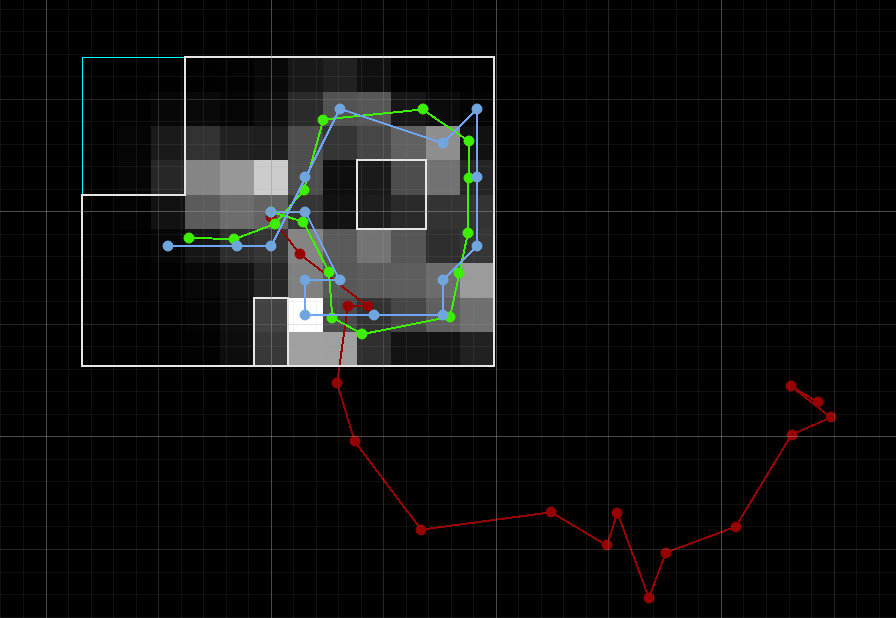
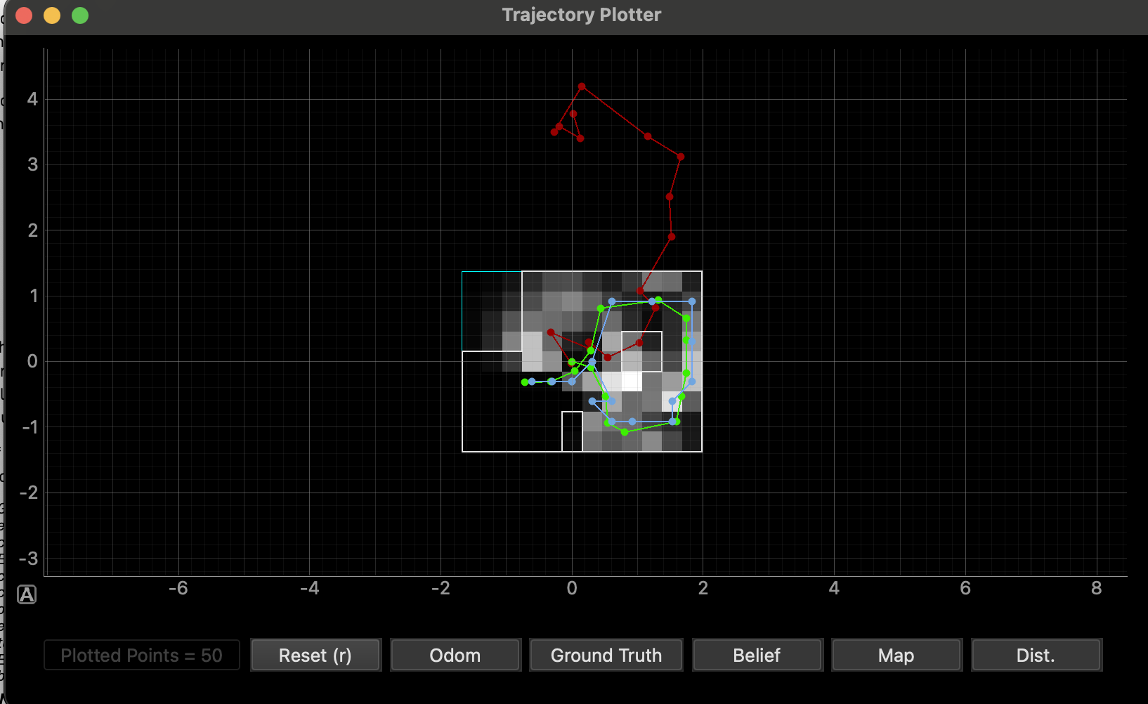
With these 5 functions completed, grid localization with Bayes Filter was complete. In order to test the functionality of this localization, a simulation is used. The simulation is split into 2 parts, being a robot display that shows the robot's behaviors, and a plotter that plots the results of the Bayes filter against the ground truth. I did two separate test runs to verify the localization behavior. Each run consists of the robot moving through a predetermined path, while computing the Bayes Filter localization to compare against this ground truth path. Moving through the path consists of the robot doing the first rotation, a translation, and then the second rotation. It then spins in a circle to collect the sensor data for the update step. This motion is in the upper left window in the videos. Then, a plotter in the lower left window shows the ground truth location (green), the Bayes Filter localization (blue), and then localization computed off of just odometry (red). The colored grids show the updating beliefs for each cell, with a lighter color indicating a higher belief. The right jupyter lab window also provides print outs for the results of each Bayes Filter step. The videos are below
Run 1 Video
Run 1 Final Graph
Run 2 Video
Run 2 Final Graph
Analysis
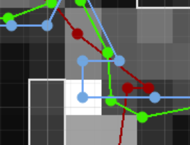
As can be seen in each of the final graphs, the blue Bayes Filter does a good job of approximating the ground truth green line. This is especially apparent when comparing against the results that occur with just using odometry, which are wildly inaccurate and inconsistent, showing the car moving outside of the actual map area in both trials. This reinforces why using a probability based model like Bayes Filter is superior to just using odometry and why localization techniques are needed. While the Bayes Filter is a good approximation, it is not perfect. A lot of the variation between the ground truth position and the Bayes estimation is due to the discritization. The Bayes filter can only have points at the center of each cell, so this inherently introduces some inaccuracy. However, even beyond this the Bayes filter would sometimes be inaccuate to the ground truth. One spot this is evident is in run 1, where after the 3rd point, the Bayes filter estimates the cell to the left, than a cell down, then a cell to the right, while the ground truth just goes down to the right.
In general, I noticed that in both runs the Bayes seemed to perform best when it was more towards the center of the map and farther away from walls, and performed worse closer to walls. Specifically, whenever the robot was near a corner seemed to perform the worst. I hypothesize that this is because there is more uncertainty within the sensor measurement when it is close to a corner like this, as it captures less of the global environment and the sensor readings are more similar to other corners nearby.
References
I referred to Mikayla Lahr's website from last year for this project, using it to help understand the different sections of this localization and debug code as well as for reference as to how to lay out the website page well. I also reviewed my final results with Giorgi Berndt.