Lab 2 - IMU
Prelab:
To prepare for this lab, I installed the 9DOF IMU Arduino Library and connected the IMU to the Artemis. I then verified this installation by running the Example1_Basics. This example had a variable called AD0_VAL, which is the value of the last bit in the device's I2C address. It is by default 1, but can be changed by closing a jumper. This I2C address must be unique from any other I2C devices accessed by the system, hence the capability to change it. I also added 3 blinks of the built in LED to indicate when the board started up.
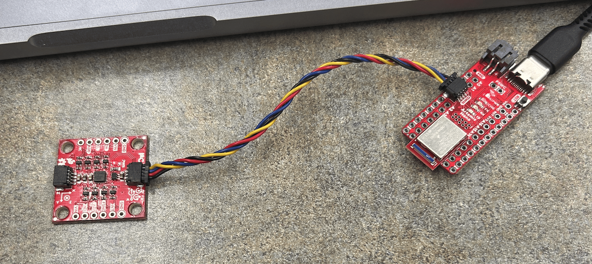
An image of the IMU setup
A video of the basic example being run, with the output shown by serial plotter
Accelerometer
In order to convert the Accelerometer into outputing pitch and yaw, the following equations from lecture were used:
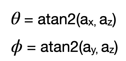
These equations have roll as about the X axis and pitch as about the Y axis. I calculated these in code using the lines:
                    pitch_a = atan2(myICM.accX(),myICM.accZ())*180/M_PI;
                    roll_a = atan2(myICM.accY(),myICM.accZ())*180/M_PI;
I then validated that 0, 90, and -90 degrees were acheivable for both pitch and roll by setting the IMU against the side of the table, as seen below:
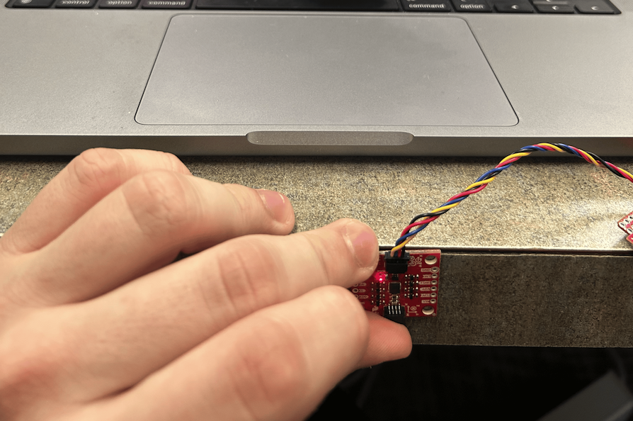
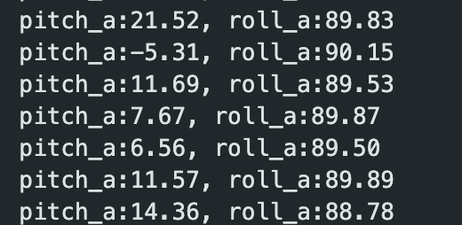
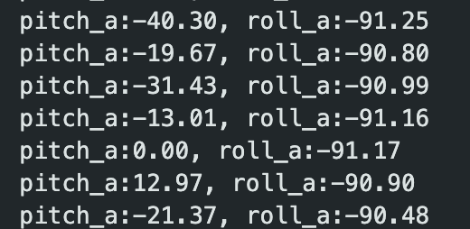
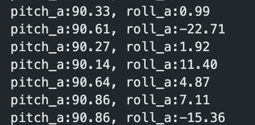
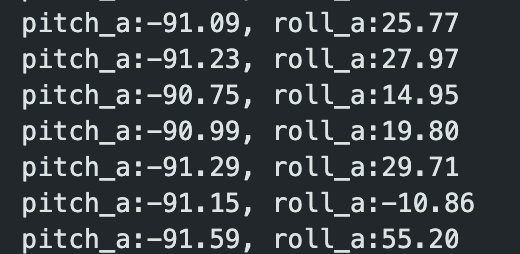
Pitch and roll at 0, -90, 90 degrees
At this point I also implemented bluetooth, so that this data would be stored in an array on a bluetooth command, and then all sent at once with another bluetootch command. I then used matplotlib to plot the readings versus time in Jupyter. The graph below is for the following video showing roll:
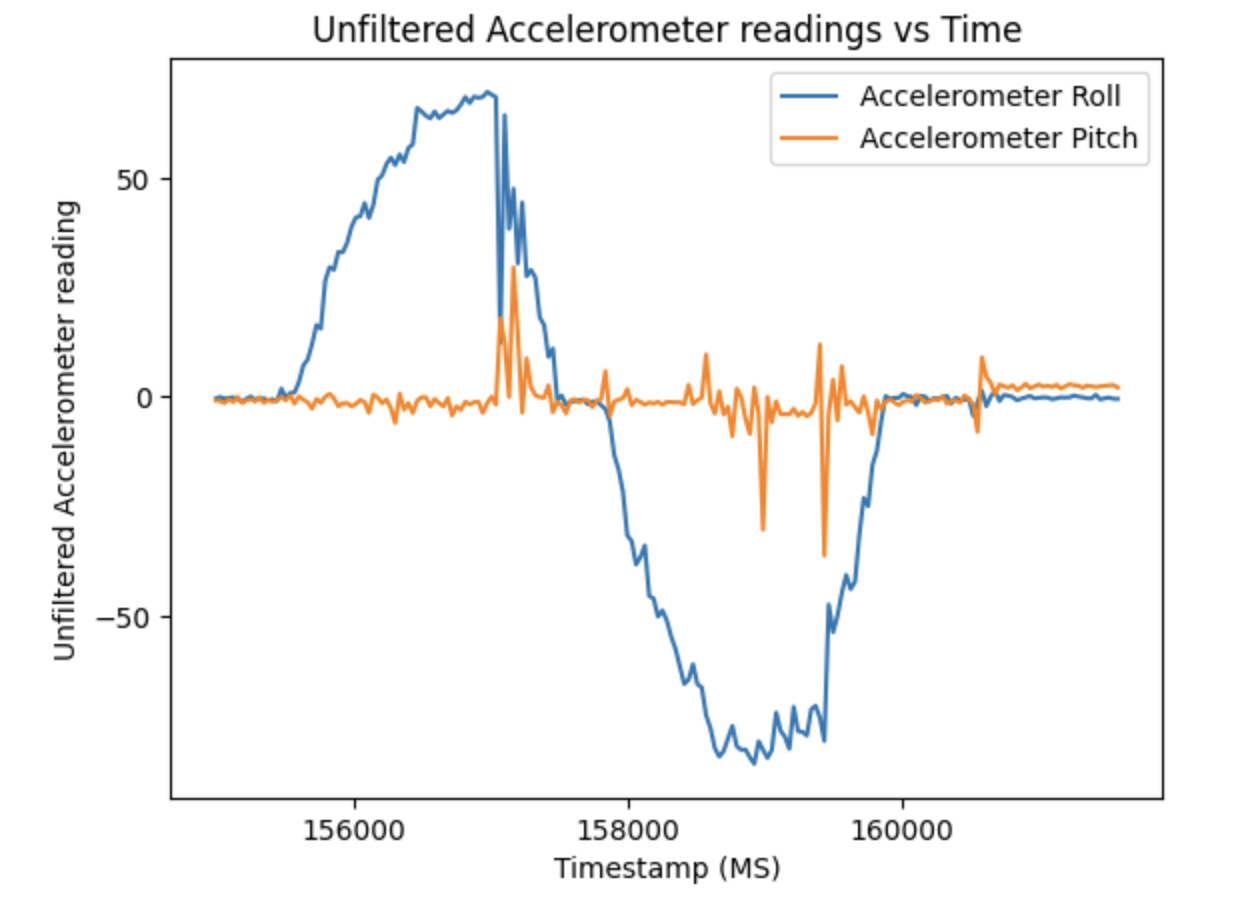
My accellerometer was initially pretty accurate, reading between -88 to 88 for roll and pitch when I put it at 90 degrees. I used the following two point correction to make the range more accurate, and validated for positive and negative 90 and 180 degrees for roll and pitch.
                    pitch_a = (((pitch_a + 88) * 180) / 176) - 90; //two point corrections
                    roll_a = (((roll_a + 88) * 180) / 176) - 90;
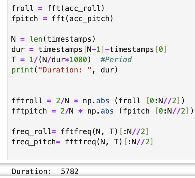
To help with noise, a Fourier Transform was used to determine a good cutoff frequency. I did my FFT in python as follows:
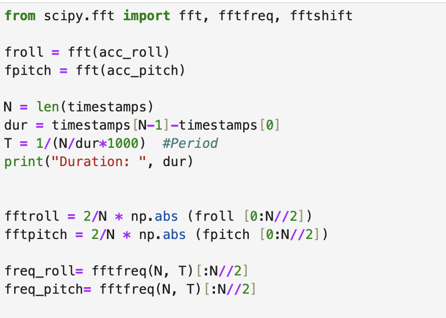
Notably, the period for it is calculated based off of the timestamps. This period could also be approximated by how long the data gathering loop delayed, which for most of this lab is 30 ms. A captured frequency spectrum for oscillating pitch is shown below:
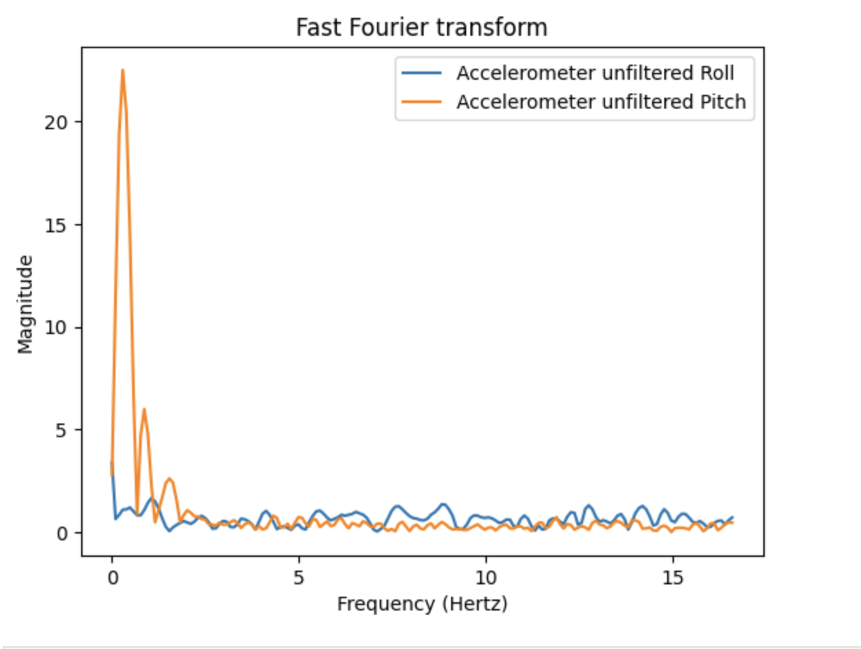
As can be seen, there is a lot of noise at the higher frequencies. I decided that the best cutoff frequency would be at the end of the largest occuring frequency, as all the other frequencies had much less magnitude. I decided for this cutoff to start at 0.5 hertz, although I also experimented with lower ones. I experimented with hitting the table to introduce more noise to confirm that this would cut off that noise, which it would. Then, a lowpass filter can be used to reduce noise. Using the RC lowpass filter equation and my cutoff frequency, I solved for an alpha value of 0.08. The following code then implements this lowpass filter.
                    //Low pass filter, about 0.25 Hz
                    //0.5 = 1/2piRC -- RC = pi
                    //alpha = T/(T+RC) -- T=30ms right now
                    const float alpha = 0.08;
                    //lowpass
                    imu_data[iter][2] = alpha*pitch_a + (1-alpha)*imu_data[iter-1][2];
                    imu_data[iter][3] = alpha*roll_a + (1-alpha)*imu_data[iter-1][3];

                    imu_data[iter-1][2] = imu_data[iter][2];
                    imu_data[iter-1][3] = imu_data[iter][3];
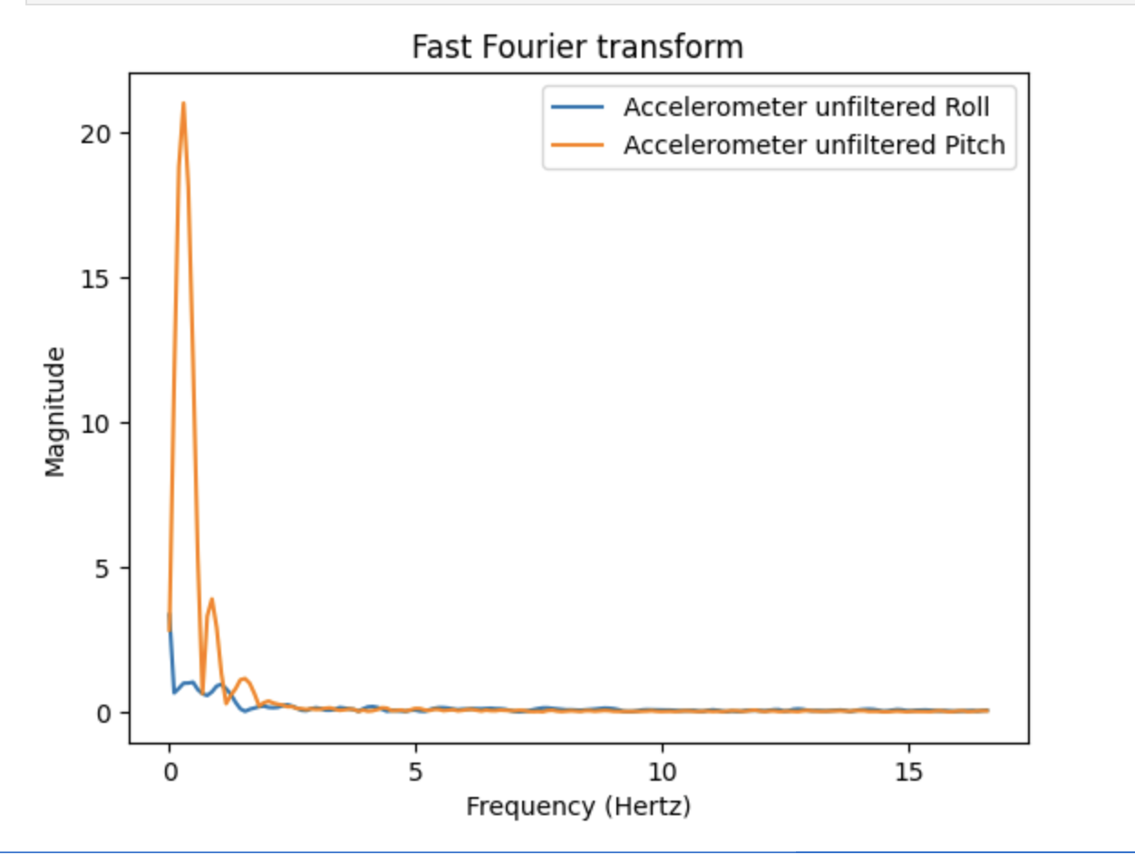
This gave the following frequency spectrum after filtering, with much less high frequency noise:
The before being filtered data and after filtering data is shown below:
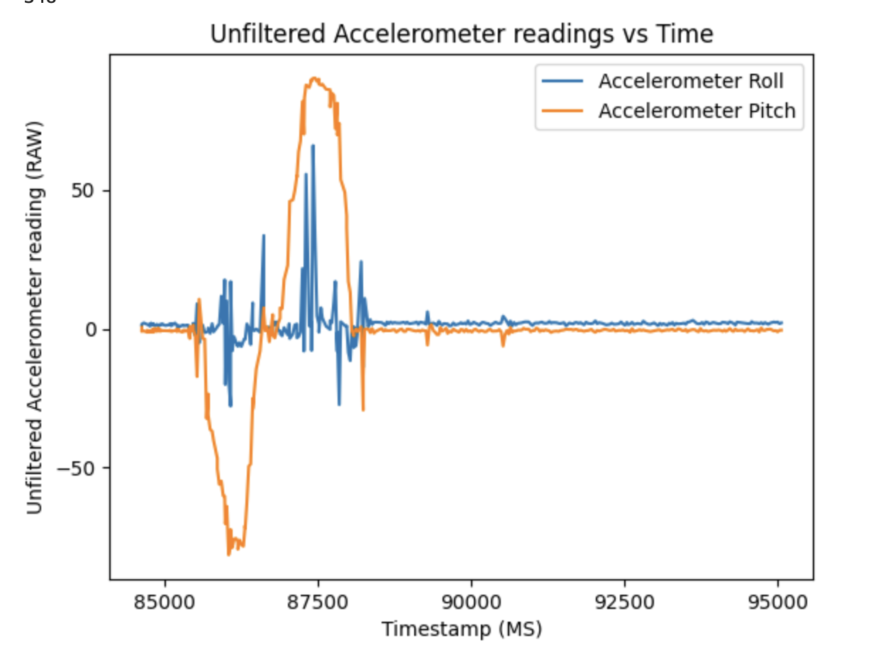
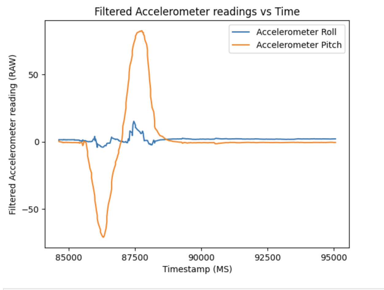
As can be seen, most of the high frequency noise is removed, and a much smoother reading is shown.
Gyroscope
In order to implement gyroscope, I used the discussed method from class of θ = θ + gyro_reading * dt. This functions by adding the gyroscope reading at each time slice to keep track of the IMU's orientation in space. This implementation is seen below:
                    dt = (micros()-last_time)/1000000.;
                    last_time = micros();
                    pitch_g = pitch_g + myICM.gyrY()*dt;
                    roll_g = roll_g + myICM.gyrX()*dt;
                    yaw_g = yaw_g + myICM.gyrZ()*dt;
To test the gyroscope, I tried rotating the sensor about each axis, producing the following graph.
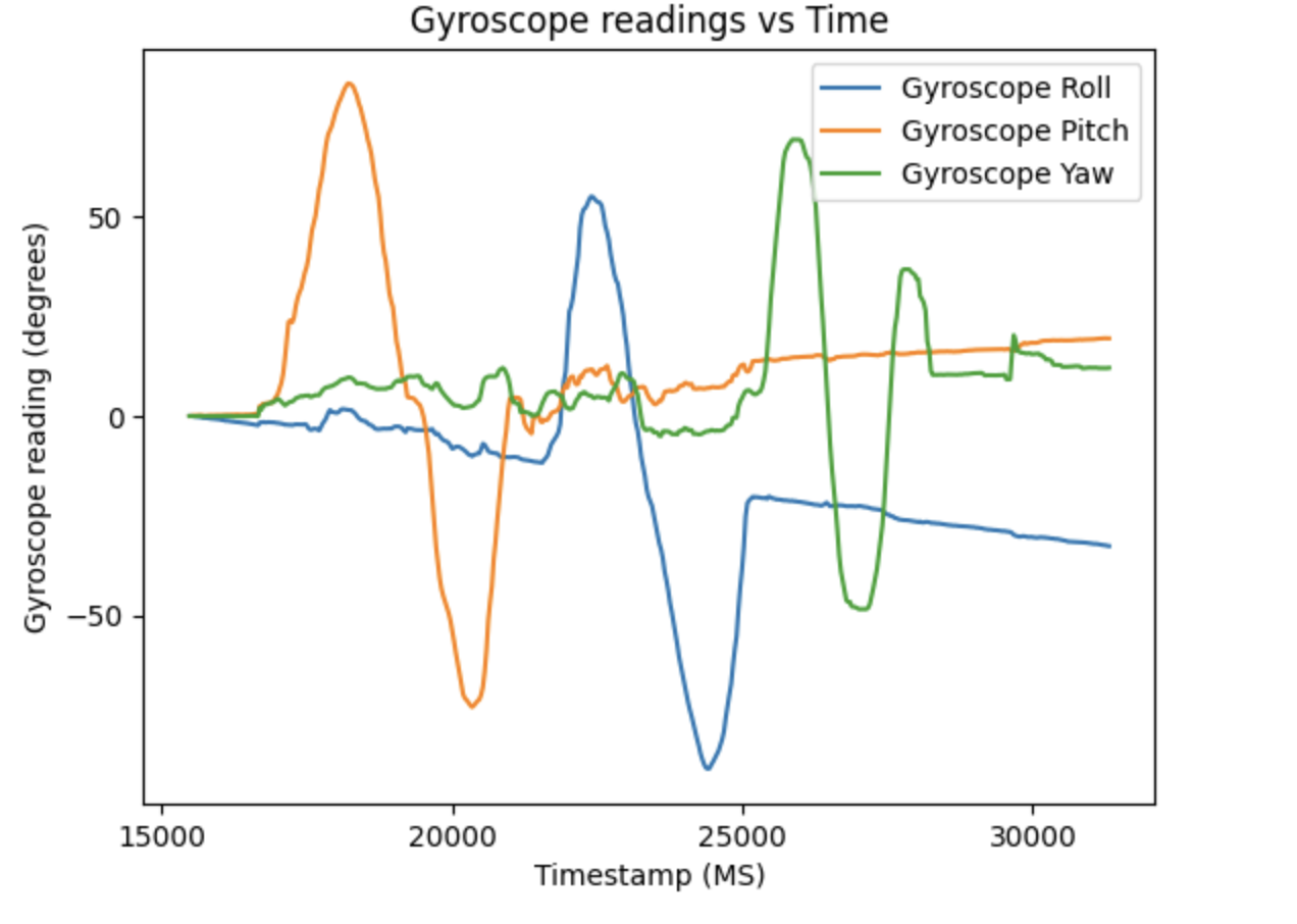
The gyroscope produced far less noisy data than the accelerometer, with most noise in this image being due to shakiness while manipulating the IMU. Each rotation is also recorded accurately in degrees, seen by the oscillations in roll, pitch, and yaw. However, the gyroscope isn't perfect as it suffers from drift, or the recorded position ending up further from the actual position of the sensor over time. This is due to how the gyroscope is tracked by accumulating readings, meaning it also accumulates error. In the above graph, this drift can be seen from roll, pitch, and yaw all not reading 0 at the end, despite the sensor being returned to the original orientation. Below is a graph of this against the accelerometer readings:
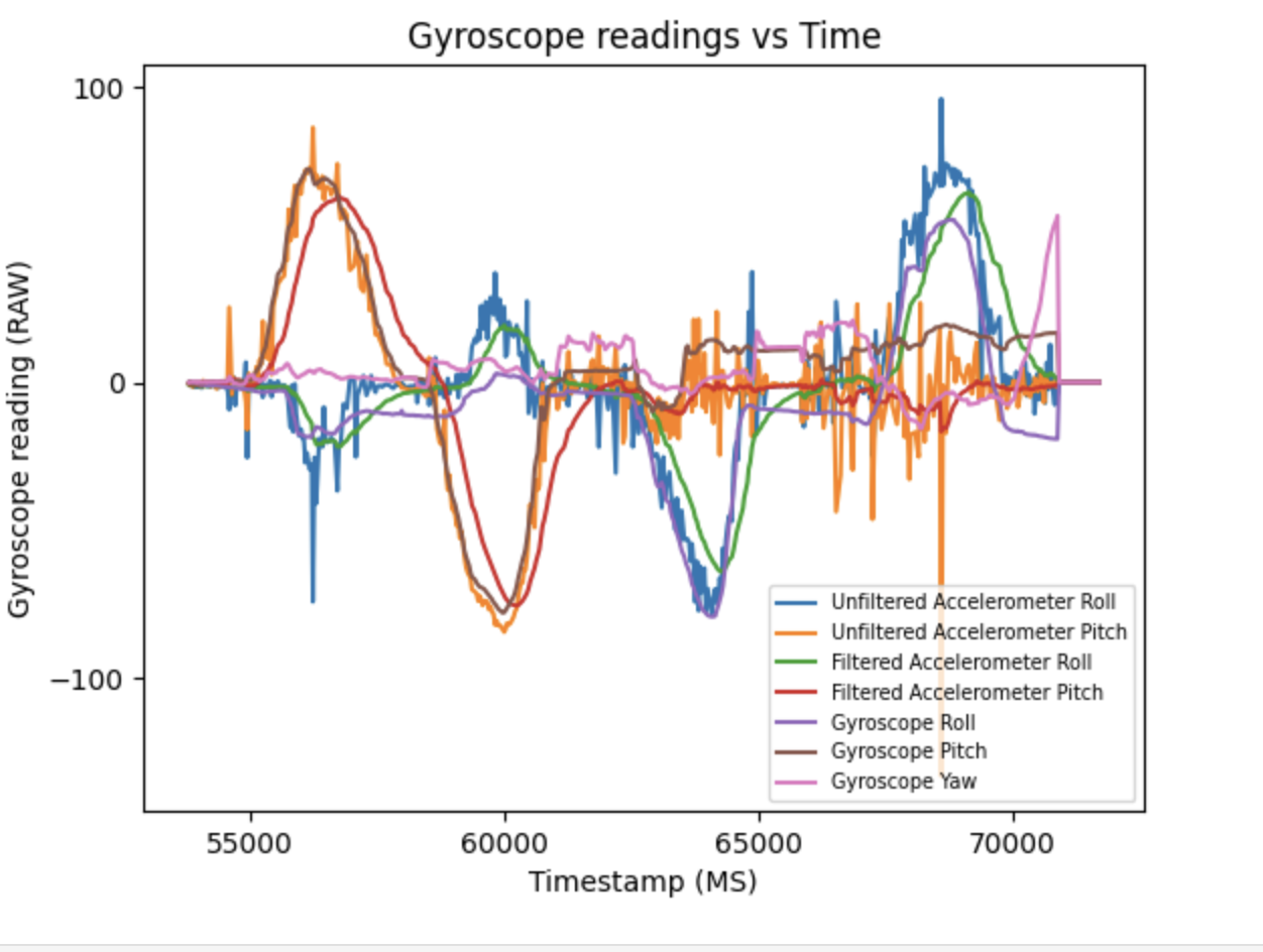
The gyroscope readings match quite nicely with the unfiltered accelerometer readings, overlapping at almost all points. The filtered accelerometer readings end up following the same pattern but not matching as nicely due to the filter prioritizing past data more than new readings, resulting in a smaller overall magnitude and the filtered data slightly trailing the gyro and unfiltered. As mentioned earlier, the gyroscope is much less noisy than the unfiltered accelerometer, but there is some drift over time observable.
Through experimentation, I found that the sampling rate of data impacted how much they gyroscope drifted. The lower the sample frequency (and thus the more time between collecting data points), the more drift that occured. I hypothesize that this happens due to having a larger dt value and less frequent gyroscope readings.
One way to overcome this shortcoming of a gyroscope is a complimentary filter. This takes advantage of accelerometers having a lot of
immediate noise, but not drifting over time, whereas gyroscopes have little noise, but experience drift. By taking a low pass filter of the
accelerometer and a high pass filter of the gyroscope, the sensors can cover each other's short comings. This was done with the equation
comp_filter[iter] = ((comp_filter[iter-1]+myICM.gyrY()*dt)*(1-alpha))+(pitch_a*alpha);. A graph produced from oscillating roll and yaw is below:
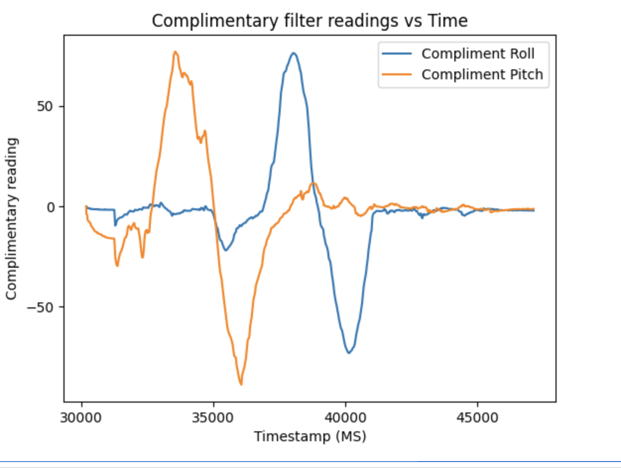
This output of data ends up being relatively smooth, with only a little bit of noise. Additionally, it appears not to drift. For better comparison, I plotted the accelerometer, gyroscope, and complimentary filter against each other.
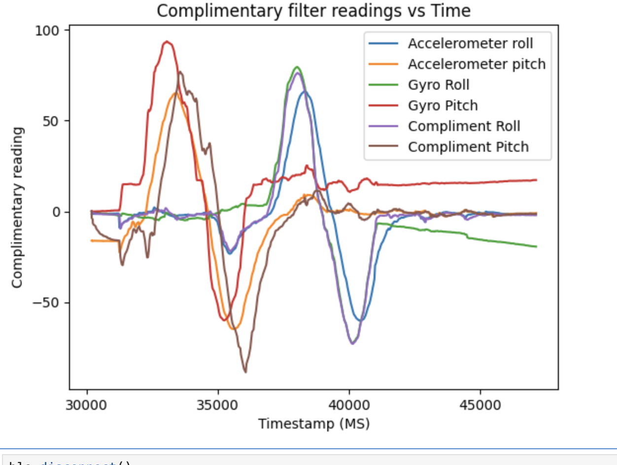
This comparison shows that there was in fact gyroscope drift that got adjusted for with the complimentary filter, seen by the filter values ending back at 0 degrees. Additionally, the noise from the accelerometer isn't present either, showing this filter is not susceptible to drift or noise. I tested the range of the sensor and found it was accurate from -180 to 180 degrees, covering the full rotation. Notably, the accelerometer data would become inaccurate and noisy when near 180 or -180, but the complimentary filter corrects for it.
Sample data
To test how the IMU would perform when sampling as fast as possible, I removed all print outs and delays from the data collection loop. Using collected timestamps, I found that the average time between data samples was 2.62 milliseconds, or a sampling frequency of 381 HZ. To allow for this, I also had to recalculate my alpha value to be 0.004, and increase the number of recorded samples. I also added a variable to count how often data wasn't ready by the time the loop returned to collect it. I found that generally the IMU could keep up with the loop, although it did end up not being ready one or two times on some runs. This suggests if my loop was even more optimized, the IMU would not keep up as well.
The way I approached storing the IMU data was to keep all the data in one large 2D array, combining the accelerometer and gyroscope readings into one spot. While this has the disadvantage of needing to allocate a large amount of contiguous memory, which could cause issues with more data, in this case it functioned without problem. I did this for ease of coding and I figured it may leverage spacial locality better, allowing for quicker memory access. However, this may not matter much for this chip, and with larger datasets I would likely break apart the arrays.
I used the float data type to store all of this data, which is 4 bytes. This allowed for more precision than would be possible with just an integer, while being more memory efficient than a string where each character is a byte or a 8 byte double. However, it may be possible to use an integer to store this data with some bit manipulation, as the higher bits of an int likely won't be used due to the degree values being relatively small. This would allow for more data storage without sacrificing much precision. With my float implementation, at most 96000 data points could be stored, although all global and local variables eat into this space. Considering that data can be collected up to once every 2.62 milliseconds, this would allow for storing 251 seconds worth of data.
To demo this higher sample rate, I increased the number of recorded samples to 2000, which allows for just over 5 seconds of recording. To verify this, I printed the total range of timestamps, which shows how many seconds the data was collected over. This came out to a bit over 5 seconds, proving the capability to record data for more extended periods.
Do a Stunt!
To end this lab, I played around with the RC car to understand it's controls and movements. I found that it drives pretty straight, and any abrupt change in direction will likely flip it. This is a good reference point for once the car is automated.
References
When working on completing the code for this lab, I discussed concepts and general ideas for implementation with Giorgi Berndt and Jorge Corpa Chunga. I also referred to the lecture notes for equations and the website of Max Freeman for formatting reference.