Lab 3 - Time of Flight Sensors

Prelab:

The goal of this lab is to set up the time of flight sensors and prepare them to be attached to the RC car for future labs. These time of flight sensors use infrared light in order to determine the distance to objects, and will be the main way that the car can percieve obstacles. Therefore, it is crucial to decide where these will be placed on the car as to give the best data. One of these sensors was decided to be at the front of the car. This was the most intuitive placement given that the car will most often be driving forward, and the sensor in front will allow for obstacles to be detected before being driven into. I considered several placements for the second sensor, including at the front at a slightly different angle for redundancy and in the rear to allow driving in reverse without hitting obstacles. Instead, I ultimately decided to place it on the right side, as later this car will be used to navigate a maze, and having the sensor on the side means that the car can check if a path exists to the right without rotating. The orientation of sensors will be as shown below.

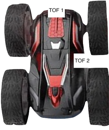
An image of the TOF sensor placement on the car

If both an obstacle is detected to the right and front in the maze, then the car will either have to make a left turn or go back the original direction, which can be determined by rotating 90 degrees. Having these sensors in this orientation will also be better for SLAM then two in front or one front one back. It has the downside of having a blindspot in the left front where obstacles could be run into, but this can be mitigated through motion planning. The sensors are angularly sensistive, so they will be placed in the middle vertically to prevent the ground from interfering with readings, whether upside down or not.

To communicate to the two IMUs, either each one had to be communicated to one at a time or the address of one needed to be changed, as they both start with the same I2C address of 0x52. I decided to change the address of one on program startup, as the other approach means data can't be gotten from both sensors simultaneously. I decided to connect each TOF to a longer QWIIC cable so they could be placed as needed on the car, while the IMU would be connected with a shorter one. The below shows the schematic I decided on for connecting these sensors:

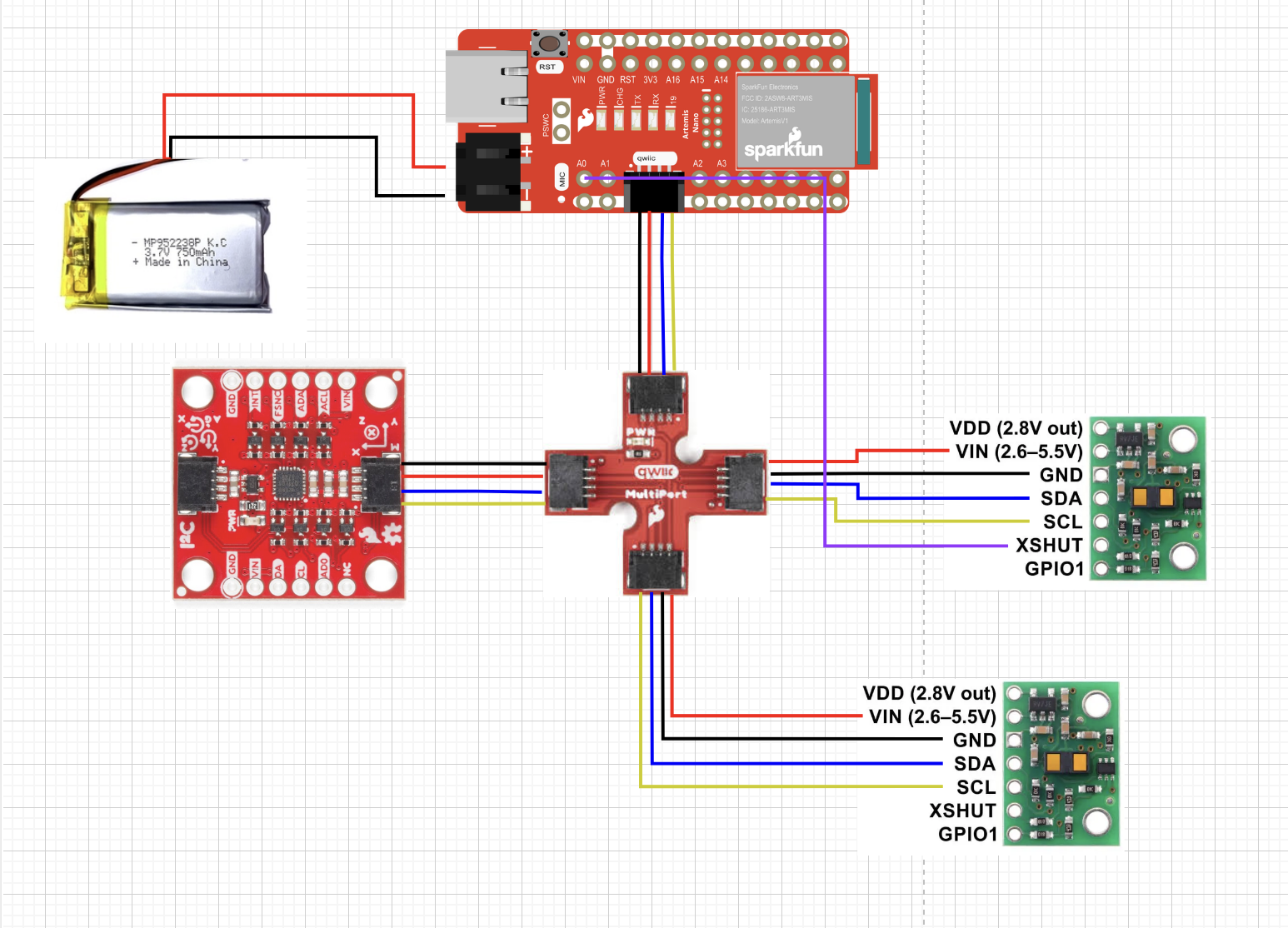
Schematic of TOF, IMU, and battery

Battery

The first step of the lab was to solder cables to the 650 mAh battery, shown below:

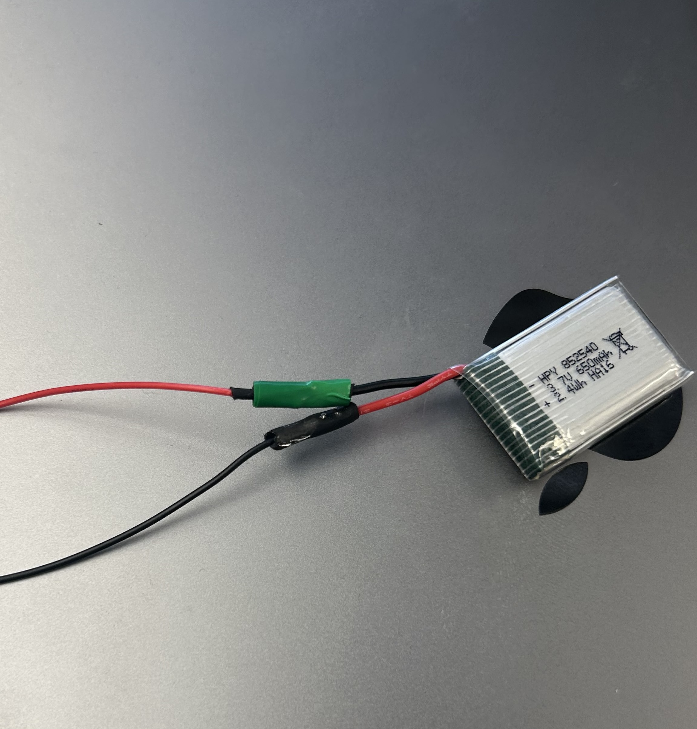
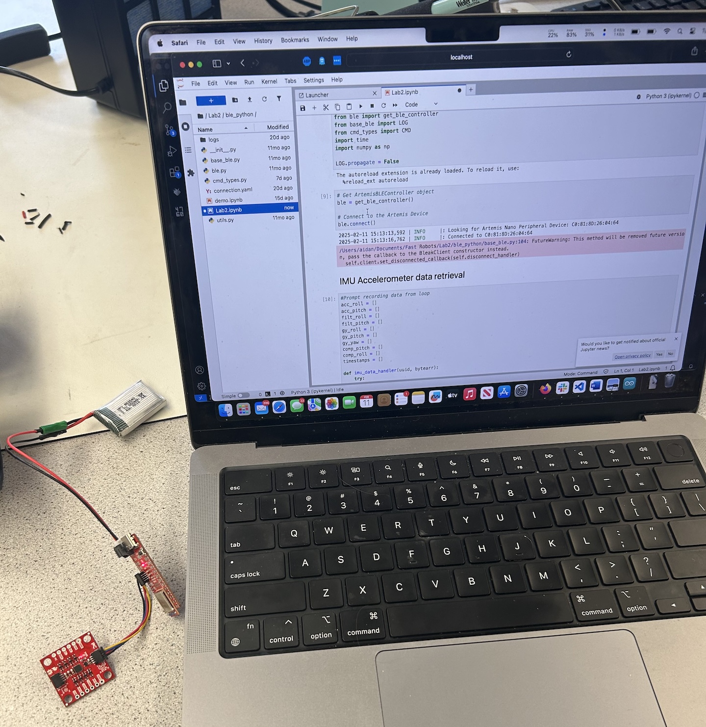
I used heat shrink to insulate each of these connections, and additionally wrapped electrical tape around one to ensure no shorts. The red and black leads end up swapped to match the Artemis Nano input port. In order to test that these connections were sound, I powered up the Artemis off of the battery with the IMU attached, and confirmed that I could still get data from the IMU via bluetooth.

First Time of Flight Sensor Setup

Firstly, I installed the SparkFun VL53L1X 4m laser distance library to interface with the TOF sensors. I then cut one of the longer QWIIC cables to allow for the sensor to be more flexible in placement, and referred to the data sheet to solder it. Specifically, blue ended up being the SDA line and yellow was the SCL line. The soldered sensor is shown below:

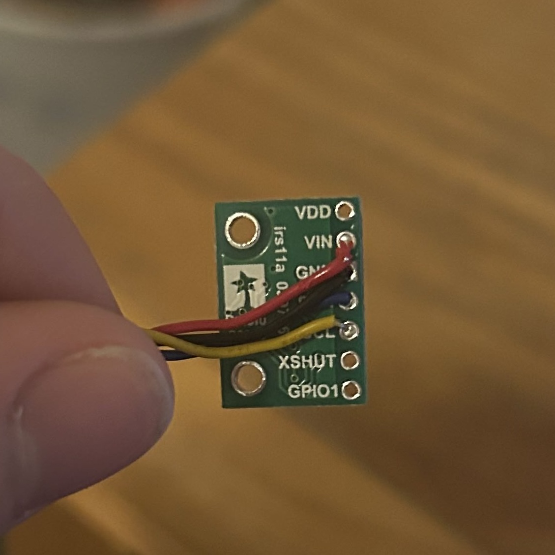
To verify that I connected this sensor correctly and that all of the solder joints were sound, I ran the Example1_wire_I2C. I connected the QWIIC port on the Artemis to the QWIIC multiport breakout, and then the TOF sensor to this breakout. Running the code gave the following:

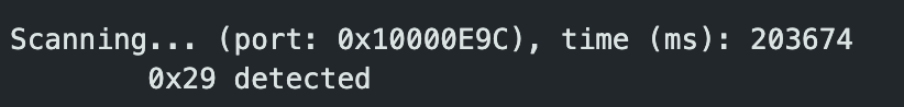
At first glance this address of 0x29 was surprising, as the datasheet for the TOF sensor said it had a default address of 0x52. However, looking at these in binary, 0x29 is 00101001 and 0x52 is 01010010, showing that the address was shifted right by one bit. This is because the least significant bit of the 0x52 address is actually used to set read or write, so the actual bts used for the i2c address are 0x29.

Time of Flight Sensor Testing

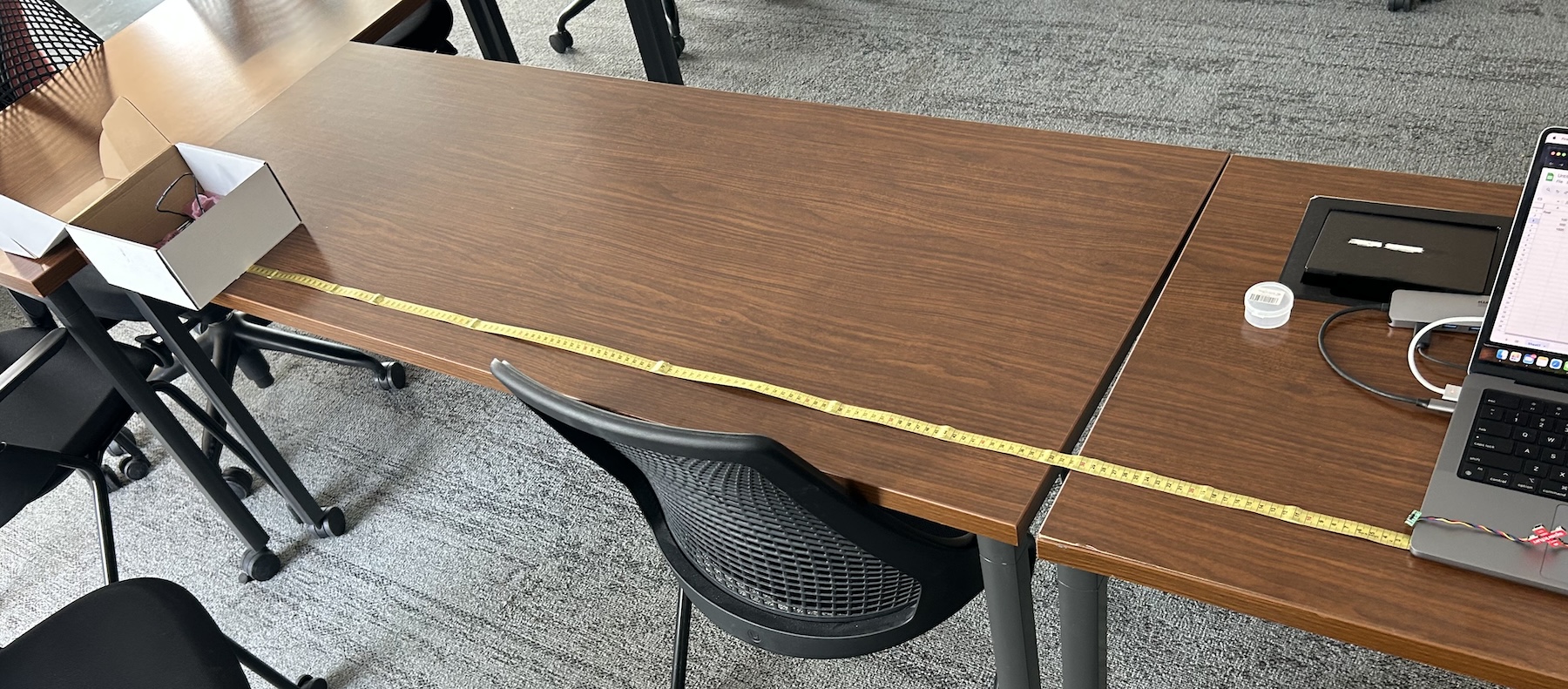
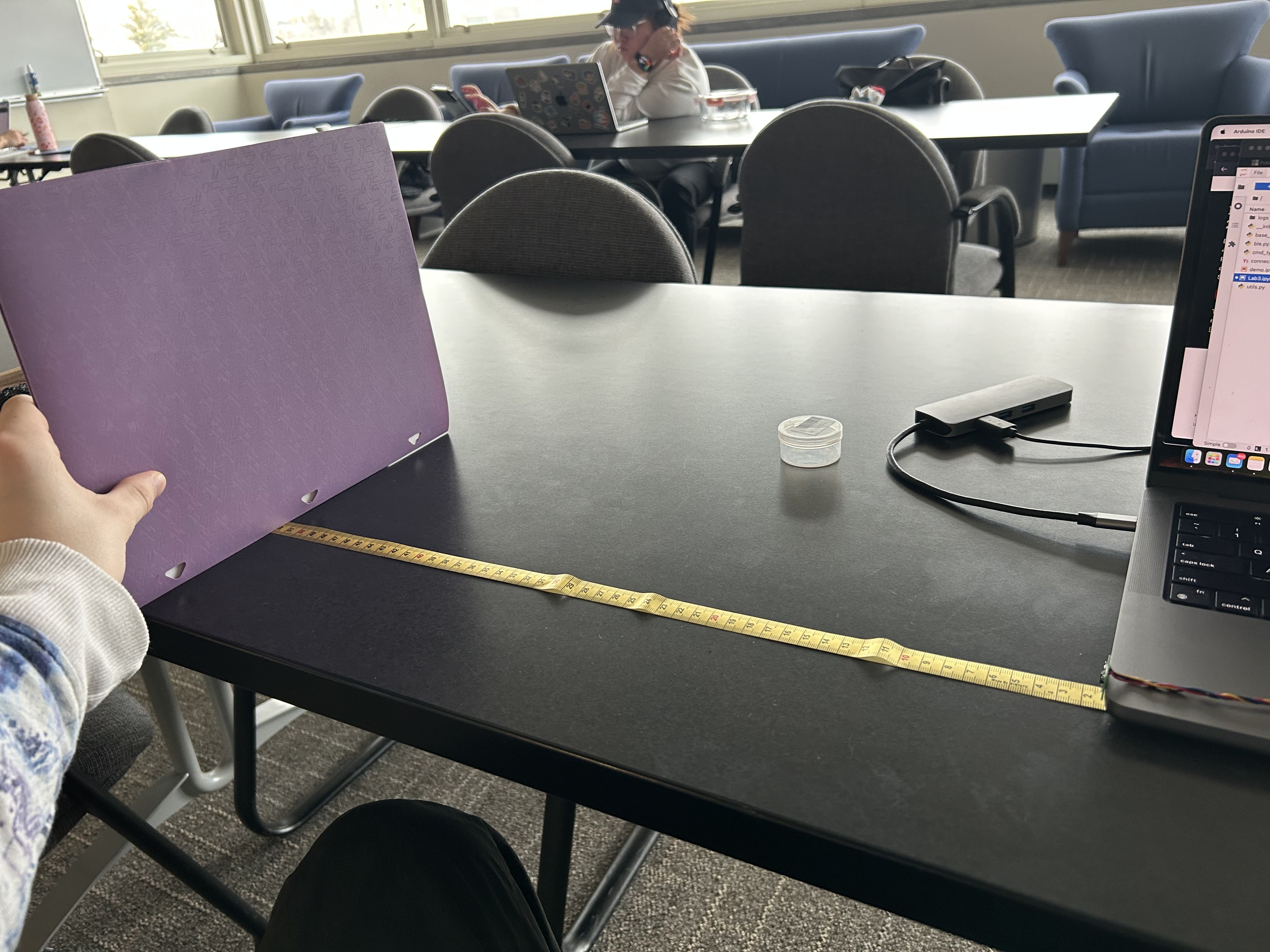
The next step was to load Example1_ReadDistance to ensure that the sensor was reading accurately. I made a setup with a measuring tape, using the provided white materials box as an object to detect and my computer to hold the sensor in one position, imaged below:

The TOF sensor could be set into several different distance modes, being short and long with tof1.setDistanceModeShort() and tof1.setDistanceModeLong(). Additionally, there was a medium mode, but this required an additional library to use. This short sensor mode is described in the datasheet as being less sensitive to ambient light but only effective to 1.3 meters, where the long would be effective to 4 meters. I decided to test both the short and long modes of the sensors between 100 millimeters and 1500 millimeters, testing for range, accuracy, and reliability. These sensor measurements were taken as averages of 256 TOF sensor readings to prove that the readings were repeatable. Notably, in the datasheet benchmarking this is done with 32 readings, but I used more to match the number of IMU readings I was taking. The below graph shows the long distance mode performance and short distance mode performance against a baseline tape measured distance.

As seen in the graph, both the long and short modes are very close to the green line, which is the tape measured distance. This validates that the sensor is accurate in both modes as well as reliable as it had many accurate readings. However, as the object gets further away, both the long and short distance modes end up slightly underestimating distance. This is more evident in the short distance sensing, with measurements past 1100 mm being short. This matches with the datasheet's discriptions of the modes.

I additionally tested the ranging time of both the short distance and long distance modes, or how long it actually took for a measurement to be made. This was accomplished with the following code, taking the difference between a timestamp when ranging starts and ends.

                    t = micros();
                    tof1.startRanging(); //Write configuration bytes to initiate measurement

                    while (!tof1.checkForDataReady()) //wait for data to be available
                    {
                        delay(1);
                    }
                    int distance1 = tof1.getDistance(); //Get the result of the measurement from the sensor
                    tof1.clearInterrupt();
                    tof1.stopRanging();

                    int elapsed = micros()-t;
                

I tested both short and long distance modes, both with the .stopRanging() and without in order to see how the ranging times vary. My results are tabulated below:

By default, the long distance mode took much longer for each individual reading, being around 90 milliseconds compared to the short range's 50 milliseconds. Additionally, removing the .stopRanging() command could save some additional time, potentially at the cost of accuracy. I also found in the datasheet that the timing budget was by default 100 milliseconds, but could be lowered to 20 milliseconds for short range and 33 milliseconds for all range. From this point on, I decided to work with the short range mode, as being able to take readings faster allows for better obstacle detection, especially at speed. Additionally, the max accurate range limitation of 1.3 meters is still reasonably large for our purposes, and the sensor can still estimate distance past that.

Second Time of Flight Sensor

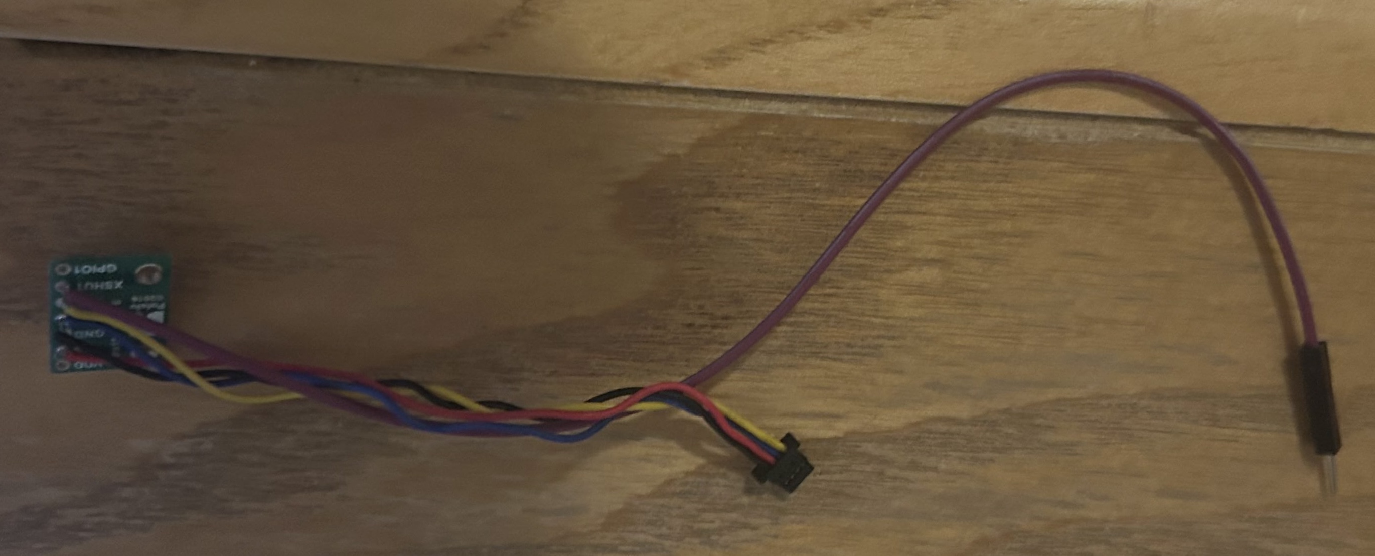
I soldered the second time of flight sensor similarly to the first, but I additionally soldered a male connection wire to the XSHUT pin and a female wire to the Artemis Nano port A0. This allows for the Artemis to control the XSHUT pin via GPIO, but makes it so the sensor isn't permanently connected to the Artemis. This may be changed later as the car design is finalized.

In order to run both sensors, on startup XSHUT needs to be held low to disable the second TOF sensor. Then, the address of the first TOF sensor is changed to 0x30 (one more than 0x29), and XSHUT is pulled high to enable the second TOF sensor. This is done in the following code.

                    #define SHUTDOWN_PIN 0

                    Wire.begin();

                    pinMode(SHUTDOWN_PIN, OUTPUT);
                    digitalWrite(SHUTDOWN_PIN, LOW); //Turn off 2nd sensor with xshut
                    tof1.setI2CAddress(0x30); //give 1st sensor different address
                    digitalWrite(SHUTDOWN_PIN, HIGH); // Turn on second sensor
                

After this, each sensor can be used with the .startRanging() and any other ranging commands simulateously without problems.

Speed of Execution

Until this point, the code reading from the sensors would delay until the TOF had data ready. However, this results in delays of 50 milliseconds or more. To avoid this, I changed the loop to check if data was ready but not block if it wasn't, timing how quick that the loop would run this way. The code is as follows:

                    tof1.startRanging(); //Write configuration bytes to initiate measurement
                    tof2.startRanging(); //Write configuration bytes to initiate measurement
                    if (tof1.checkForDataReady())
                    {
                      int distance1 = tof1.getDistance(); //Get the result of the measurement from the sensor
                      tof1.clearInterrupt();
                      tof1.stopRanging();
                      Serial.print("Distance1(mm): ");
                      Serial.println(distance1);
                    }
                    if (tof2.checkForDataReady())
                    {
                      int distance2 = tof2.getDistance(); //Get the result of the measurement from the sensor
                      tof2.clearInterrupt();
                      tof2.stopRanging();
                      Serial.print("Distance2(mm): ");
                      Serial.println(distance2);
                    }
                  
                    Serial.print("Loop time (ms): ");
                    Serial.println(millis());
                

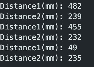
Running this gave the following output:

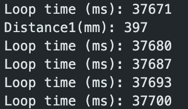
The loop averaged taking only 7 milliseconds to complete this way, being roughly the same whether or not sensor data was available. This is much faster than the delay method. Likely, this loop would run even faster, but the Serial print outs used to display the loop time are probably taking significant time. If the serial prints were removed, then the next bottleneck would likely be that I am repeatedly restarting ranging, which may not be necessary.

Bluetooth and IMU integration

The next step was to integrate these sensors with the BLE and IMU from Lab 2. I connected all of the sensors together via the QWIIC multiport, resulting in the following setup:

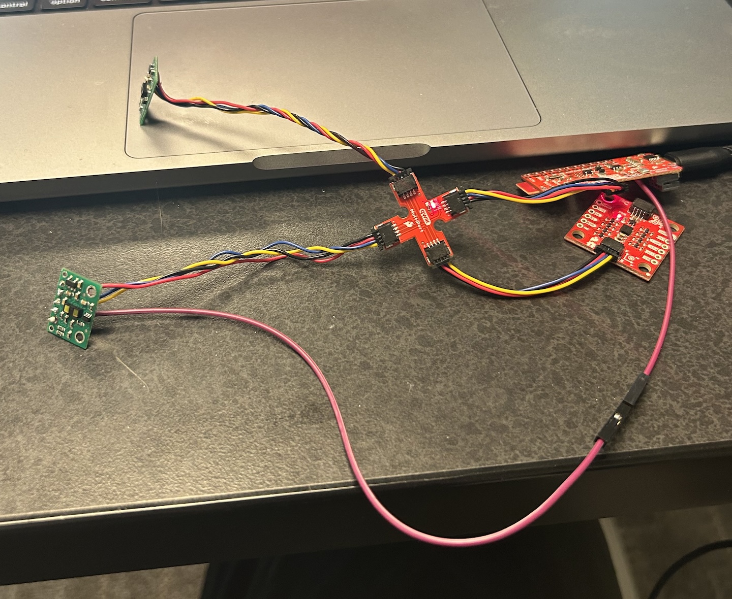
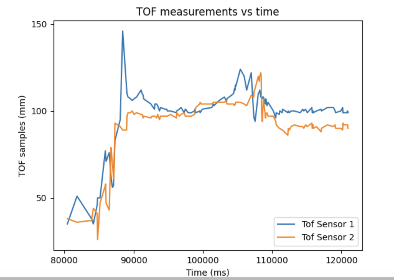
I leveraged the same data collecting flag from lab 2 which would trigger both the IMU and TOF to collect data. I used the above nonblocking TOF sensor readings to collect data in the main loop() function, just before IMU data would be collected. The TOF data for each sensor was stored in a 2XN int array, separate from the IMU data. I also had separate timestamps for the TOF as the IMU would collect data faster than the TOF, so the timestamps wouldn't line up. 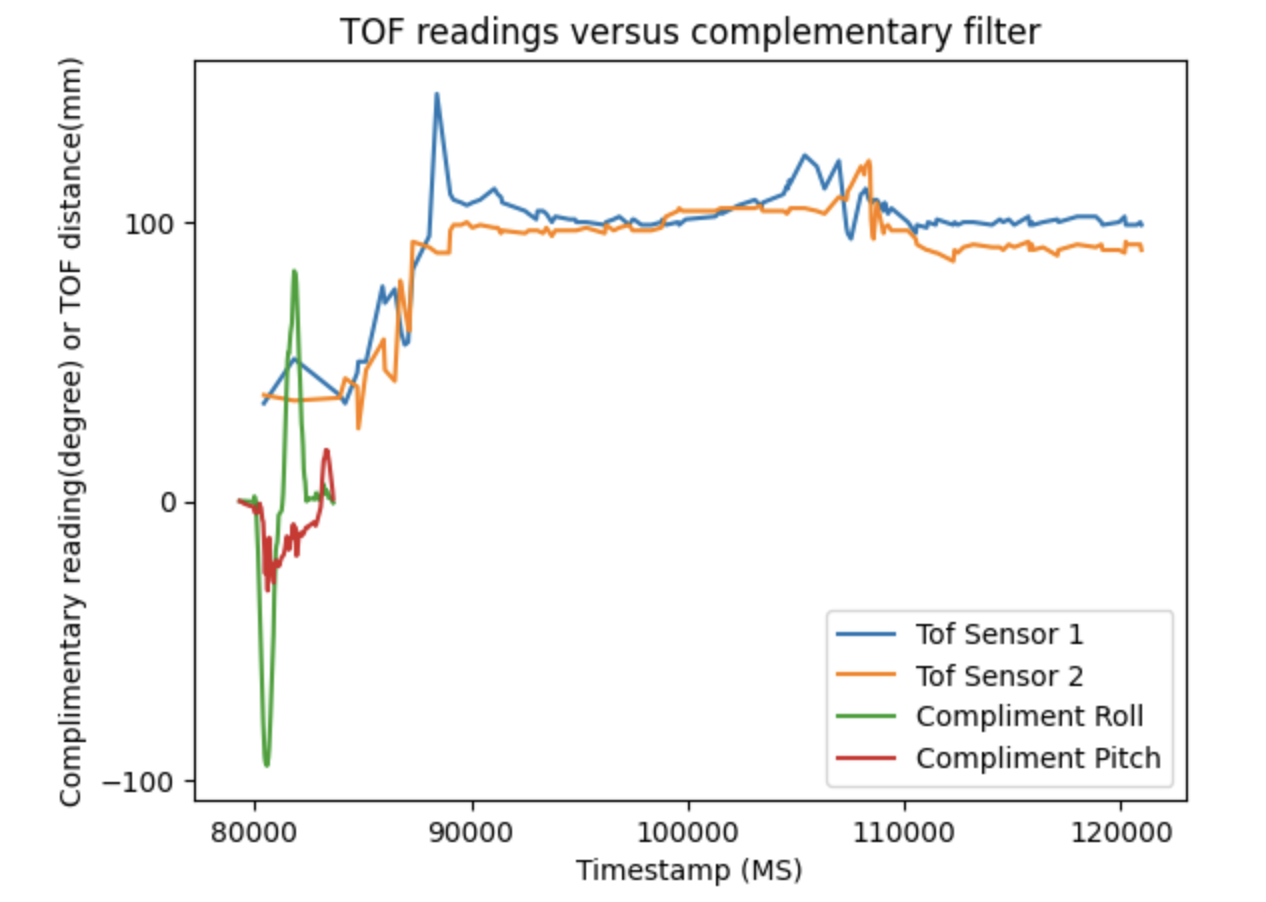I added a command GET_TOF_DATA to transfer this data over BLE. With this, I recorded TOF data vs time for both sensors:

Here is the IMU complementary filter sensor data measured at the same time:

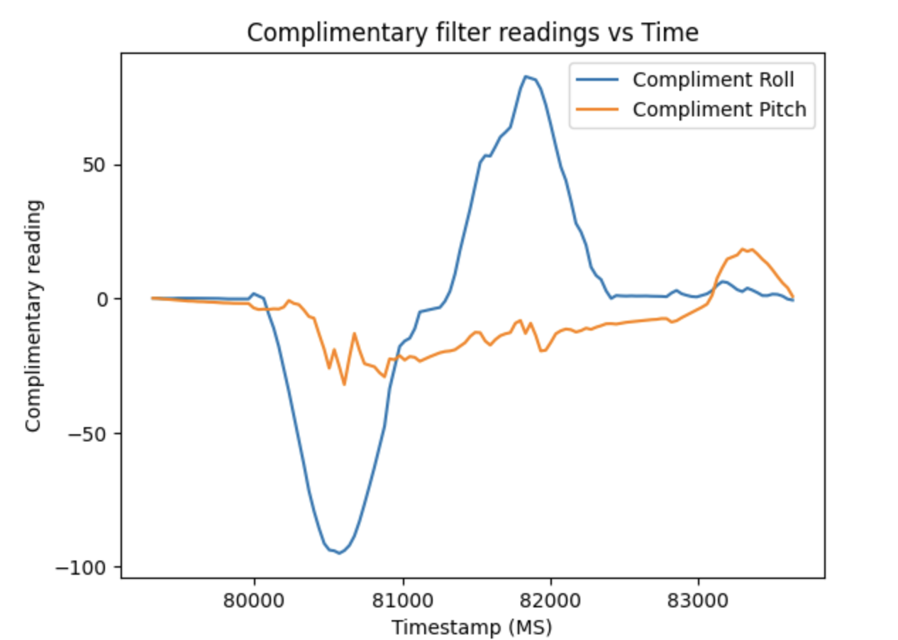
The next graph shows both the complementary filter IMU adata and TOF data plotted on the same graph to prove they were captured simulataneously. The IMU colllects all of its datapoints much faster than the TOF, although the timing budget hasn't been minimized yet.

5000 Level Questions

There are a few different ways to measure range when using Infrared rays, such as our TOF sensors. There are both passive and active infrared sensors, where the passive sensors measure IR from the environment whereas the active emit IR rays and measure the reflection of the ray. Passive sensors are convenient in that they are low power, but cannot accurately measure distance, mainly being used in systems like proximity detectors that dont require exact ranges. In the actice infrared category, there are both TOF sensors and infrared distance sensors. The TOF sensor emits a pulse of IR light and measures the time it takes to return to get range, while other infrared sensors just measure reflected intensity. This make TOF more accurate and generally with larger ranges, but the other sensors are more affordable and better for low cost environments.

As the TOF sensor fundamentally functions on IR waves, its performance is dependent on what exactly it is detecting. In order to explore this, I measured several different colors and materials each at 500 millimeters to see how the reading would change.

The following table displays these results:

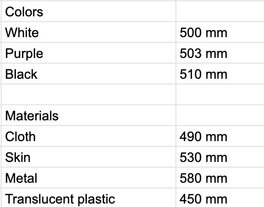
There were only very subtle differences in different colors, but they were not the same. In my experimentation, white materials produced the closest to the measured value, with black being the furthest off, and other colors being in between. This makes sense, as it means the black is likely absorbing more of the infrared light. However, I did find that material had a significant impact on distances. Cloth was very similar to the solid cardboard or plastic I was using for colors, but skin ended up being off by 30 millimeters. Interestingly, transluscent plastic seemed to result in underestimates. However, the most interesting is when I had used metal, the sensor was off by 80 millimeters. Notably, for both the transluscent plastic and metal, the object I was using were circular, so this may also be hurting accuracy.

Overall, this shows its important to be mindful of the environment the sensor is used in. Specifically, solid, flat, matte surfaces seem to be the best, especially if they are white.

References

When working on completing the code for this lab, I discussed concepts with Giorgi Berndt and Jorge Corpa Chunga. I also referred to the various datasheets and provided examples for the TOF.