Lab 6 - Orientation control
Lab 6's goal is to take the PID controller designed in Lab 5 and adjust it to allow for PID control for the car's orientation. This uses the IMU to get the current angle of the car compared to the desired set point.
Prelab:
Bluetooth:
When starting this lab, a few extra bluetooth cases were added. Firstly, a "ORIENT" command was added that started the car turning to a target angle. This just set a flag to indicate to the main loop to run the orientation code and reset the start time and an index for tracking data.
                    case ORIENT:
                    {
                      mycar.orient = 1;
                      mycar.start_time = millis();
                      mycar.e_pos = 0;
                      break;
                    }
Additionally, since the orientation control and position control will eventually happen simultaneously, and each will have different KP, KI, and KD values, a separate command was set to help tune the orientation constants, shown below.
                    case SET_OPID:
                    {
                        float P, I, D;

                        success = robot_cmd.get_next_value(P);
                        if (!success)
                          return;

                        success = robot_cmd.get_next_value(I);
                        if (!success)
                          return;

                        success = robot_cmd.get_next_value(D);
                        if (!success)
                            return;
                        mycar.OKP = P;
                        mycar.OKI = I;
                        mycar.OKD = D;
                        break;
                    }
One major difference between this lab and Lab 5 is that the setpoint will no longer be constant. To let the set point to be changed while driving, the Bluetooth command SET_TARGET was added, setting both the distance and orientation setpoints.
                    case SET_TARGET:
                    {
                      float dist_targ, orient_targ;
                      success = robot_cmd.get_next_value(dist_targ);
                      if (!success)
                        return;

                      success = robot_cmd.get_next_value(orient_targ);
                      if (!success)
                        return;
                      mycar.dist_target = dist_targ;
                      mycar.orient_target = orient_targ;
                      break;
                    }
Eventually, the decisions of set points can be automated fully for an application like navigating a maze or doing a stunt, needing to change while driving. By setting this command to change targets while driving this functionality can be tested. All of the above commands are callbacks from the BLE interrupting the system, allowing for them to be run while the system is still driving. Additionally, the setpoint was added to the data that would be transmitted to Python, with the below Python notification handler recieving and parsing the string of data.
                    prop = []
                    time = []
                    motor = []
                    dist_targ = []
                    orient_targ = []
                    def pid_data_handler(uuid, bytearr):
                        try:
                            piddata = ble.bytearray_to_string(bytearr)
                            arr = piddata.split("Prop:")[1] #Split messages
                            prop1, arr = arr.split("Motor:")
                            motor1, arr = arr.split("Time:")
                            time1, arr = arr.split("dist:")
                            dist, ang = arr.split("ang:")
                            prop.append(int(prop1))
                            motor.append(int(motor1))
                            time.append(int(time1))
                            dist_targ.append(int(dist))
                            orient_targ.append(int(ang))
                        except Exception as e:
                            print(e)


                    ble.start_notify(ble.uuid['RX_STRING'], pid_data_handler)
This data was retrieved with the GET_PID command. In its current implementation, this can't be ran while driving as it will send all the recorded data over at once, blocking the PID loop from running. These values could all be plotted in Python once transmitted.
Lab:
Digital Motion Processor - Yaw:
The yaw calculated in Lab 2 was an integral of the gyroscope measurements, with the line yaw_g = yaw_g + myICM.gyrZ()*dt;
calculationg the angular velocity over a time step for find orientation. However, this integration will also accumulate error over each
measurement, leading to the gyroscope drifting over time. This can be offset by using a complementary filter, taking a high pass of the gyroscope
reading and low pass of the accelerometer to make a more stable reading. However, this still can drift slightly over longer time. Thus, the IMU's built
in Digital Motion Processor (DMP) was used in order to calculate the yaw. The DMP performs a more sophisticated integral of the gyroscope readings
with other sensors to return high quality quaternions that are less subject to drift. It also accounts for slight offsets on other axis, which is ideal as
there is no way to guarantee the IMU is perfectly level.
This was implemented following the Fast Robot DMP Tutorial:
                    void get_DMP() {
                    // Is valid data available?
                      if ((myICM.status == ICM_20948_Stat_Ok) || (myICM.status == ICM_20948_Stat_FIFOMoreDataAvail)) {
                          // We have asked for GRV data so we should receive Quat6
                          if ((data.header & DMP_header_bitmap_Quat6) > 0) {
                              double q1 = ((double)data.Quat6.Data.Q1) / 1073741824.0; // Convert to double. Divide by 2^30
                              double q2 = ((double)data.Quat6.Data.Q2) / 1073741824.0; // Convert to double. Divide by 2^30
                              double q3 = ((double)data.Quat6.Data.Q3) / 1073741824.0; // Convert to double. Divide by 2^30

                              double q0 = sqrt(1.0 - ((q1 * q1) + (q2 * q2) + (q3 * q3)));

                              double qw = q0; // See issue #145 - thank you @Gord1
                              double qx = q2;
                              double qy = q1;
                              double qz = -q3;

                              // yaw (z-axis rotation)
                              double t3 = +2.0 * (qw * qz + qx * qy);
                              double t4 = +1.0 - 2.0 * (qy * qy + qz * qz);
                              double yaw = atan2(t3, t4) * 180.0 / PI;
                              mycar.yaw = yaw;
                          }
                      }
                    }
Only the yaw was calculated by this function as it is used as theta, minimizing the calculations occuring in PID loop. This
function is called only when the orientation control is running. The code myICM.readDMPdataFromFIFO(&data); is read
every loop however, as otherwise the FIFO buffer will fill up and cause the program to run out of memory and crash. The rate of the
DMP can be controlled so data doesn't come in faster than it is retrieved. In the setup() function, several functions from the DMP
tutorial are called to initialize it. The gyroscope still has some limitations, with the maximum angular velocity it can record being
plus or minus 2000 degrees per second (dps). There are also modes for 250, 500, and 1000 dps, which can be set in code. This is ample for
this application, as the car will never spin that fast in one second. I set this to the max of 2000 with the line success &= (IMU.enableDMPSensor(INV_ICM20948_SENSOR_GAME_ROTATION_VECTOR) == ICM_20948_Stat_Ok);
The sampling speed of the IMU could also hypothetically be a limit, but in this instance it samples at 1.1 KHz, which was plenty for
this use case. The PID loop running with DMP and the new orientation code runs at 13 ms per loop on average, although there was some variance,
likely from when TOF data is collected. Whatever angle the IMU is at when it is initialized is considered 0 degrees by the DMP.
PID Control:
PID control was used for this orientation control due to it allowing for the most customizability and already being mostly implemented from Lab 5. It was easy to integrate this with a yaw measurement from the IMU, with the PID code being identical, and only the function arguments changing to pass angle measurements, setpoints, and constants.
                    float calc_pid(int dist, int setpoint, float KP = mycar.SKP, float KI = mycar.SKI, float KD = mycar.SKD, float alpha = 0.9) {
                        //proportional terms
                        int e = dist-setpoint;

                        //log info
                        mycar.e_hist[mycar.e_pos] = e;
                        mycar.t_hist[mycar.e_pos] = millis();
                        mycar.target_hist[mycar.e_pos][0] = mycar.dist_target;
                        mycar.target_hist[mycar.e_pos][1] = mycar.orient_target;
                        mycar.e_pos ++;

                        mycar.I += e * float(mycar.dt)/1000; // integral term
                        if(mycar.I > 1000) {
                          mycar.I = 1000;
                        }
                        else if (mycar.I < -1000){
                          mycar.I = -1000;
                        }


                        if (mycar.e_pos >= PID_LENGTH) { //Loop logs
                          mycar.e_hist[0] = mycar.e_hist[PID_LENGTH-2];
                          mycar.e_hist[1] = mycar.e_hist[PID_LENGTH-1];
                          mycar.t_hist[0] = mycar.t_hist[PID_LENGTH-2];
                          mycar.t_hist[1] = mycar.t_hist[PID_LENGTH-1];
                          mycar.motor_hist[0] = mycar.motor_hist[PID_LENGTH-2];
                          mycar.motor_hist[1] = mycar.motor_hist[PID_LENGTH-1];
                          for(int i = 2; i < PID_LENGTH; i++) {
                            mycar.e_hist[i] = 0;
                          }
                          mycar.e_pos = 2;
                        }

                        if (mycar.e_pos > 1) { //Derivative turn
                          float d = (mycar.e_hist[mycar.e_pos-1] - mycar.e_hist[mycar.e_pos-2]) / (float(mycar.dt)/1000);
                          mycar.dF = d*alpha + (1-alpha)* mycar.dF;
                        }
                        else {
                          mycar.dF = 0;
                        }

                        return KP*e + KD*mycar.dF + KI*mycar.I; //PID sum
                      }
A new function for turning the car was added to allow differential drive. This ran the motors in opposite directions to have the car spin in place. In order to overcome static friction, a value of 140 PWM is written for 30 ms, before allowing the speed to drop down to the actual value. The value passed into this drive was clipped between 166 and 110, with 110 being the slowest it could turn and 166 times the scaling being the max value. All future graphs of motor value show the calculated motor speed from PID, not the adjusted one for the sceond motor.
                if (value > 0) {
                    //startup to avoid deadband
                    if(sign(mycar.last_drive) != sign(value) && value < 130) {
                      analogWrite(MOTORLF, 140);
                      analogWrite(MOTORRB, 140*adjust);
                      analogWrite(MOTORLB, 0);
                      analogWrite(MOTORRF, 0);
                      mycar.deadtime = millis();
                      Serial.println("Deadband Start");
                    }
                    else if(millis()-mycar.deadtime > 30) {
                      analogWrite(MOTORLF, value);
                      analogWrite(MOTORRB, value*adjust);
                      analogWrite(MOTORLB, 0);
                      analogWrite(MOTORRF, 0);
                      Serial.println("Deadband End");
                    }
                  }
                  else {
                    if(sign(mycar.last_drive) != sign(value) && value > -130) {
                      analogWrite(MOTORLB, 140);
                      analogWrite(MOTORRF, 140*adjust);
                      analogWrite(MOTORLF, 0);
                      analogWrite(MOTORRB, 0);
                      mycar.deadtime = millis();
                    }
                    else if(millis()-mycar.deadtime > 30) {
                      analogWrite(MOTORLB, -1*value);
                      analogWrite(MOTORRF, -1*value*adjust);
                      analogWrite(MOTORLF, 0);
                      analogWrite(MOTORRB, 0);
                    }
                  }

                  mycar.last_drive = value;
                }
To calibrate the constants, I started with KP, keeping KI and KD at 0. Since I want the full speed of 166 when the error was 180 degrees, KP was calculated to be 166/180 degrees as a starting value, or 0.9222. After experimenting with several other values, I found that a KP value of 0.9 worked the best, producing the following video when the target was set to 90 degrees:
Duct tape was added to the wheels to help the car turn in place smoother. The graphs of the angle of the car, the set targetpoint, and the motor control is shown below:
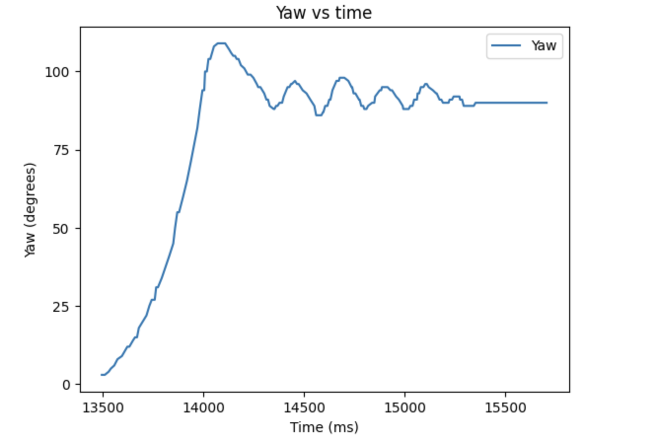
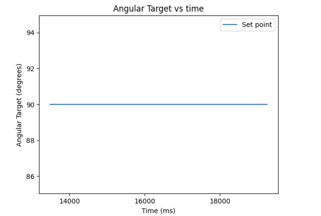
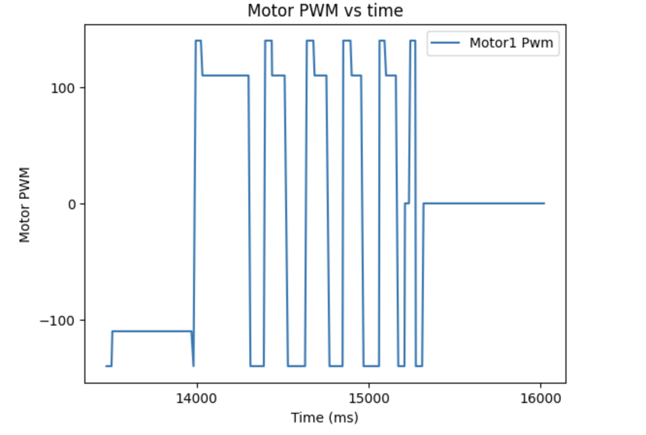
P Control Yaw (degrees), Target Angle (degrees), and Motor Output
These images reflect how the robot oscillated around the target point of 90 before stopping. The motor output shows how the output could be put up to 140 or -140 to overcome static friction, and how it has a deadband of 110 and -110.
Derivative:
The derivative term for the orientation control is interesting, as the proportional term is the integral of angular velocity. Thus, the derivative is close to calculating the angular velocity by undoing the integral. However, it is different since it is the derivative of the error between the current location and desired location, meaning it gives the rate of change of error. This is useful for helping to prevent overshoot and help it react to changing a setpoint. By testing KD with KI at 0 and KP at 0, I lowered it from 0.016 until the system was stable, getting a value of 0.008.
To test whether this actually helped with overshoot, I set my setpoint to -180 so the motors would speed up more. This also tested if the KP was well calibrated, and would cause a control of 166 when 180 degrees away. One issue is that the DMP can return negative or positive yaws. This means that the controller can wrap around from -180 to positive 180. If this happens, the current controller spins a full circle to get back to -180. The PID loop was made to always take the most optimal route to a target angle by ensuring the error term is always between -180 and 180, seen below:
                    if(mode == 1) { //Check in orientation mode
                        if(e > 180) { //indicates its better to go around the other way
                            e -= 360;
                        } else if(e < -180) {
                            e += 360;
                        }
                    }
The following video demonstrates that the car can now move to the -180 degree target and stabilize there with PD control.
The following are the graphs from this run:
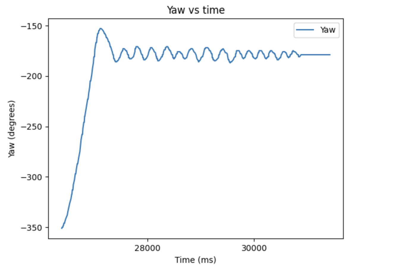
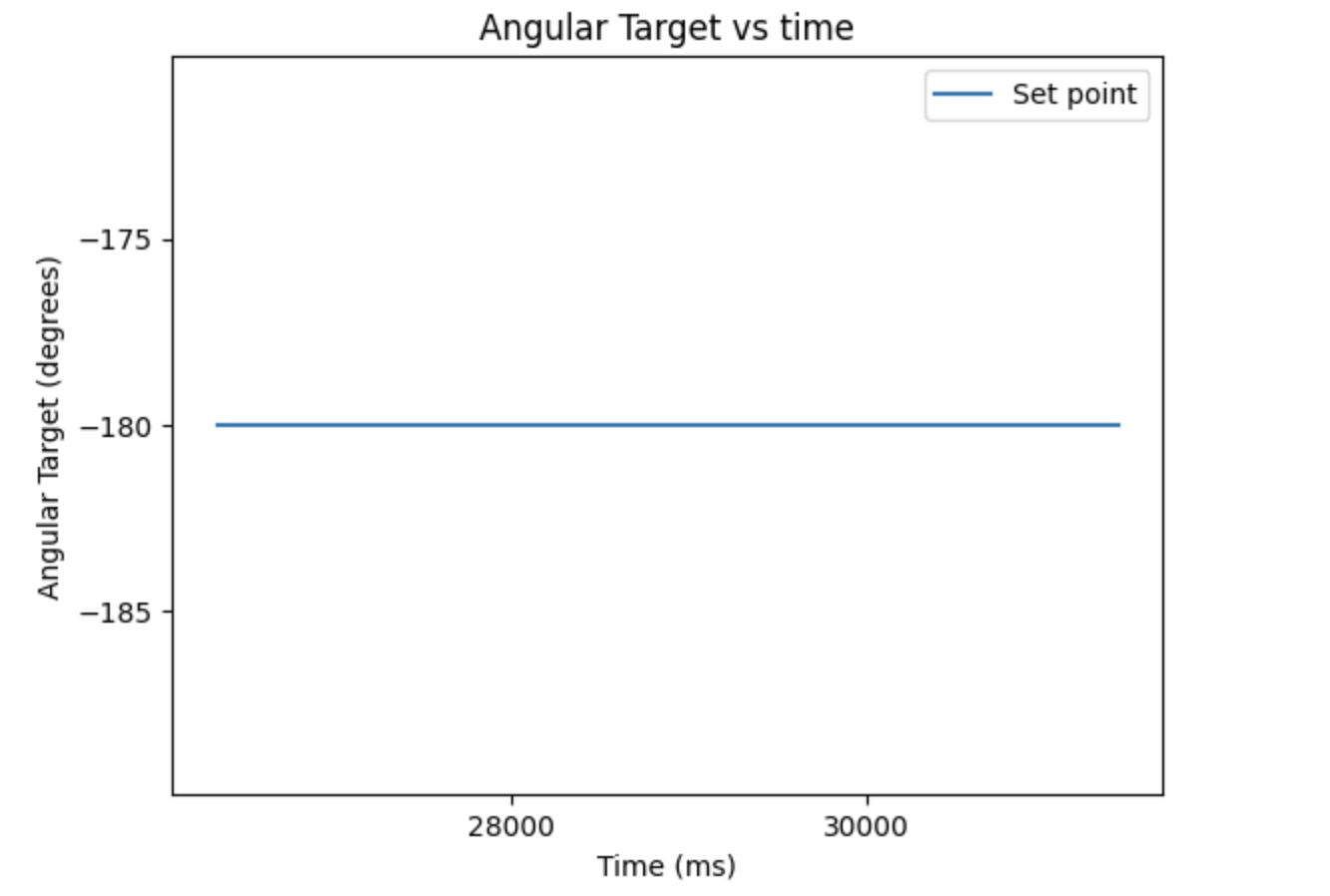
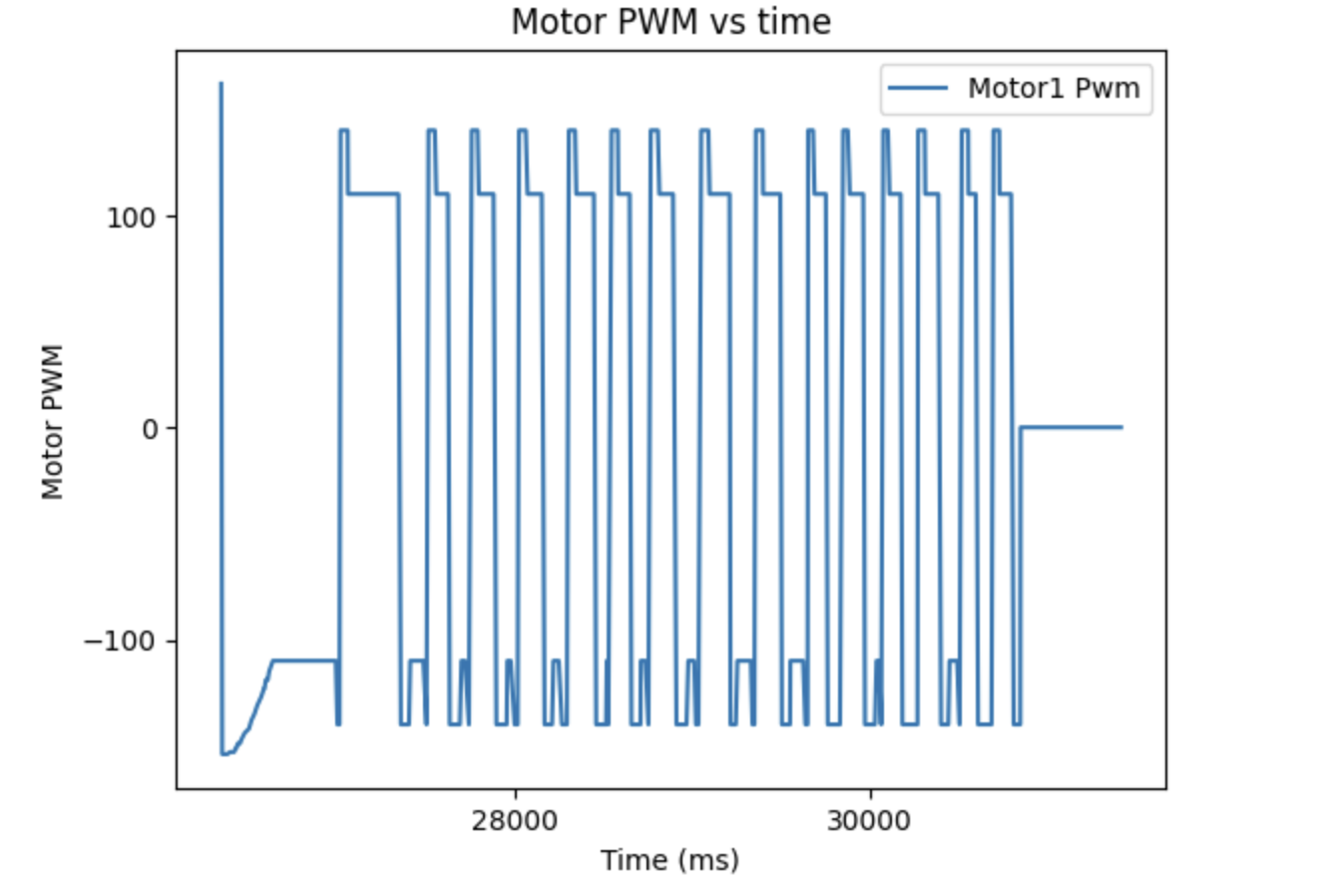
PD Control Yaw (degrees), Target Angle (degrees), and Motor Output
Notably, the overshoot for the yaw is minimized by the derivative term and the oscillations are relatively small. The motor control also shows that KP is large enough to build up the motor speed when it is 180 degrees from the target.
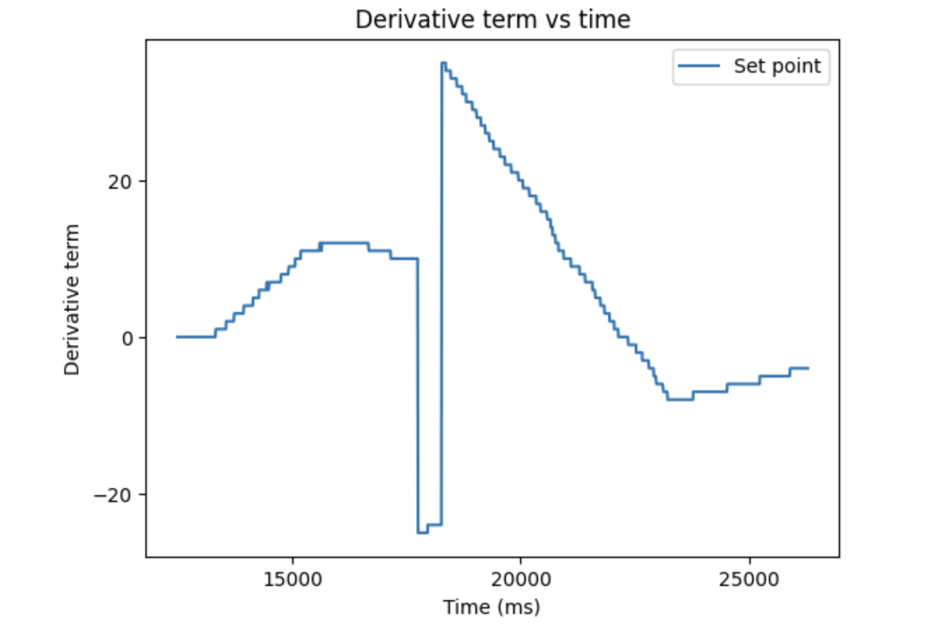
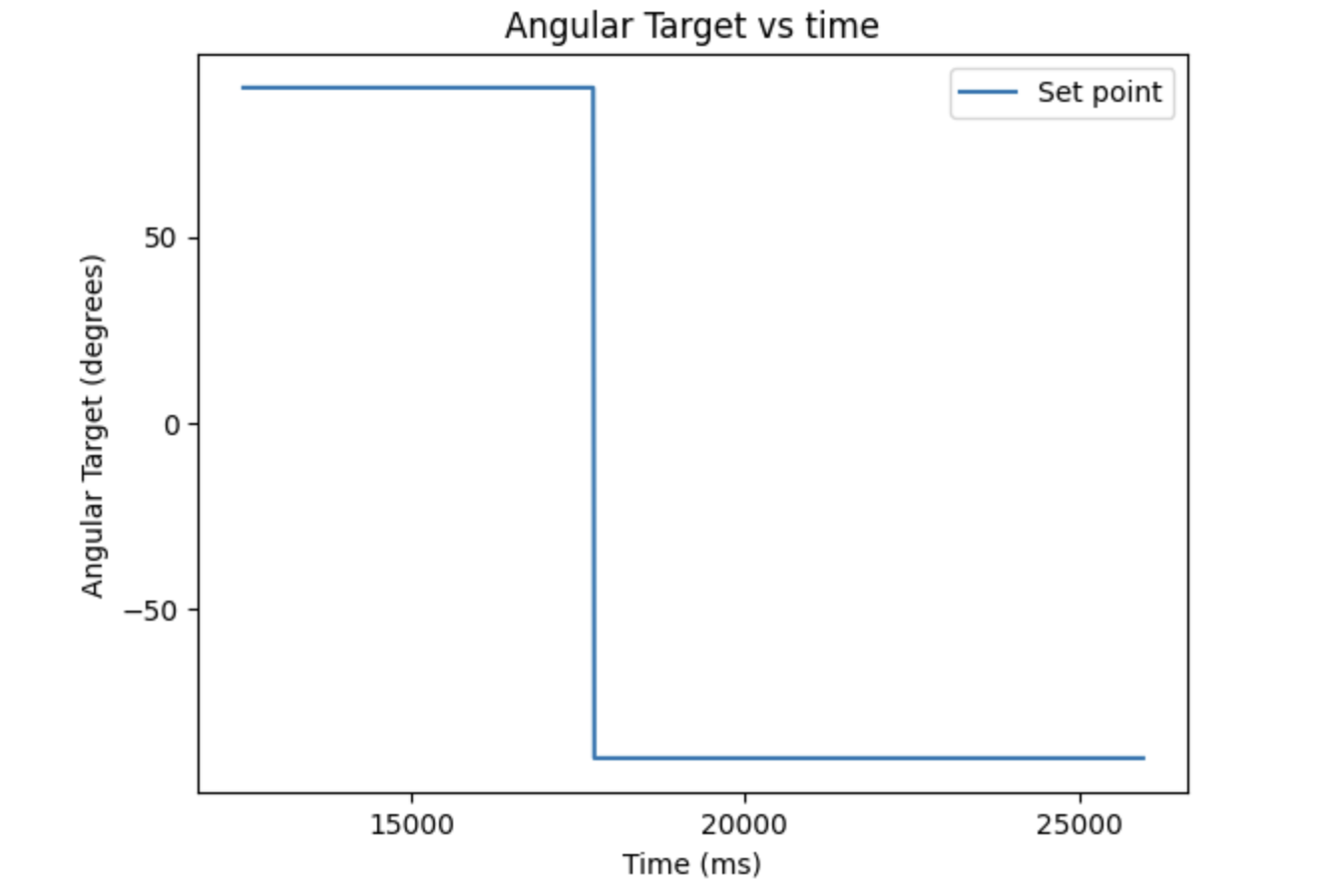
Since the setpoint can be changed, derivative kick is an issue. This is when changing the setpoint caused the derivative term to spike due to a large change in error, which will cause the motor driver to be run at a very high speed right when the swap occurs. This is shown below.
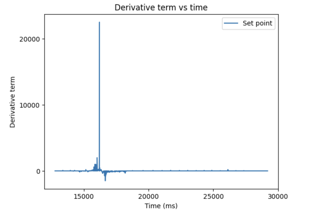
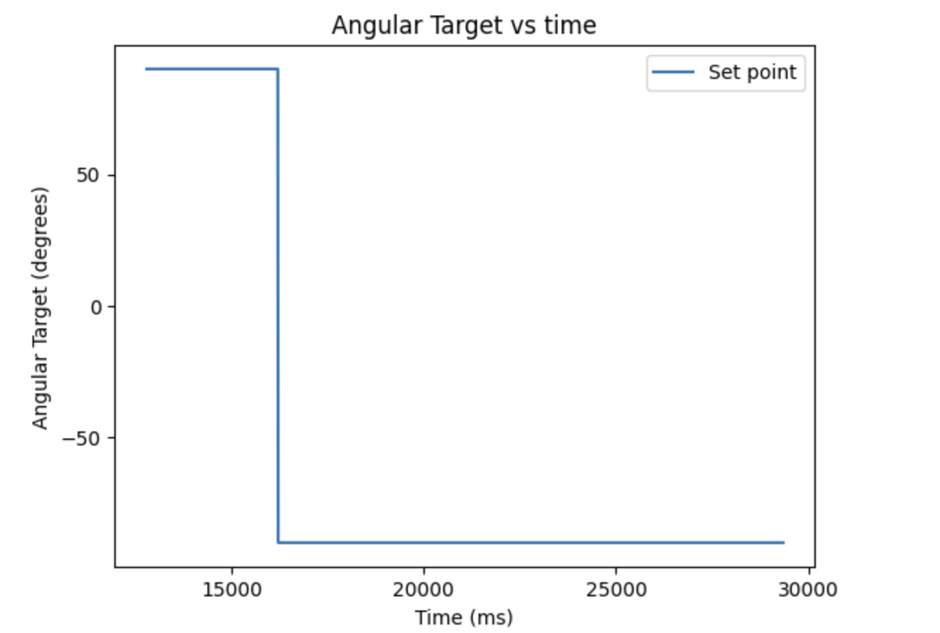
Derivative kick and Set point shift
There are several ways to deal with this, but I did it by taking a lowpass filter on the derivative term to prevent a high frequency spike like this.
mycar.dF = d*alpha + (1-alpha)* mycar.dF;
The term alpha determines how much low pass filter passes, with a low alpha blocking most high frequencies by heavily weighting past dFs. An alpha of 0.002 was chosen as it gave the best performance, eliminating most of the magnitude of the spike while still allowing the derivative term to change at a reasonable rate.
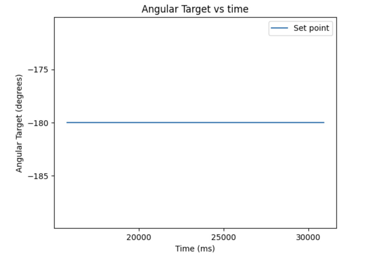
Derivative lowpass and Set point shift
Integral:
The integral term was then implemented to help with steady state error, which could be caused by differing surfaces. In order to properly test it, I put my car on an uneven surface, being my backpack. Without any integral term, the below is the following performance:
The proportional control term and derivative term are not forcing the motors to high enough speeds to actually turn on this uneven surface. I tested several values both against this surface and the ground to make sure the I value wasn't too high, finding a value of 0.1 to be the best performing, seen below on the backpack.
The integral winds up enough to finish the turn, producing the following graphs:
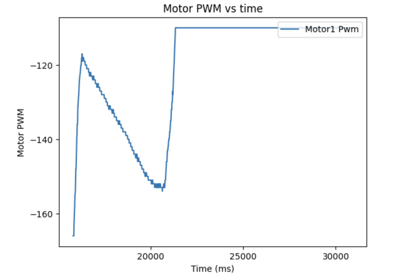
PID Control Yaw (degrees), Target Angle (degrees), and Motor Output
The motor control shows how the integral term winds up overtime to force the car to move, while dropping once the car overcomes whatever obstacle.
Changing Setpoint:
With the PID controller done, the last step was to test how it behaved when the set point was changed mid run. I had it start at a setpoint of 90 and swap to -90 to demonstrate that the car could react and converge on the second set point.
This video shows that the car can in fact change the setpoint in live time and react, reaching and oscillating around both setpoints. One note is there was a decent amount of overshoot and it oscillated more instead of converging. This was due to the earlier calibration being done on carpet, and the lower friction of the smooth floor with the tape making the car slide more. Without the tape or with different calibration this could be reduced. The graphs for this run are below.
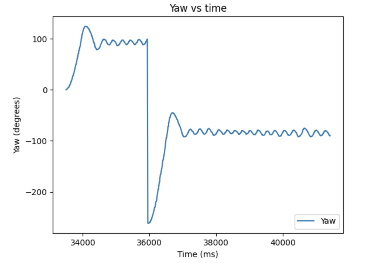
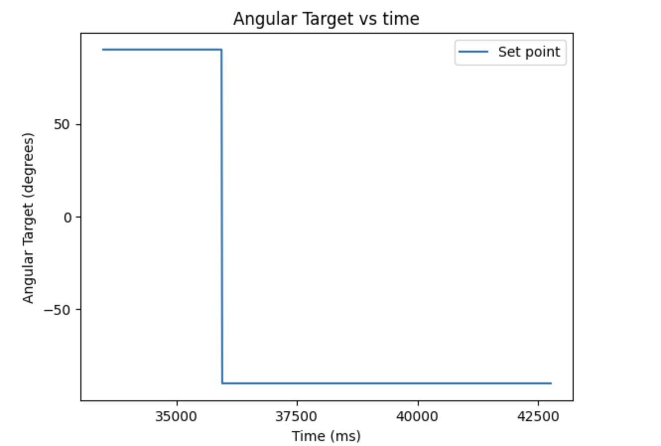
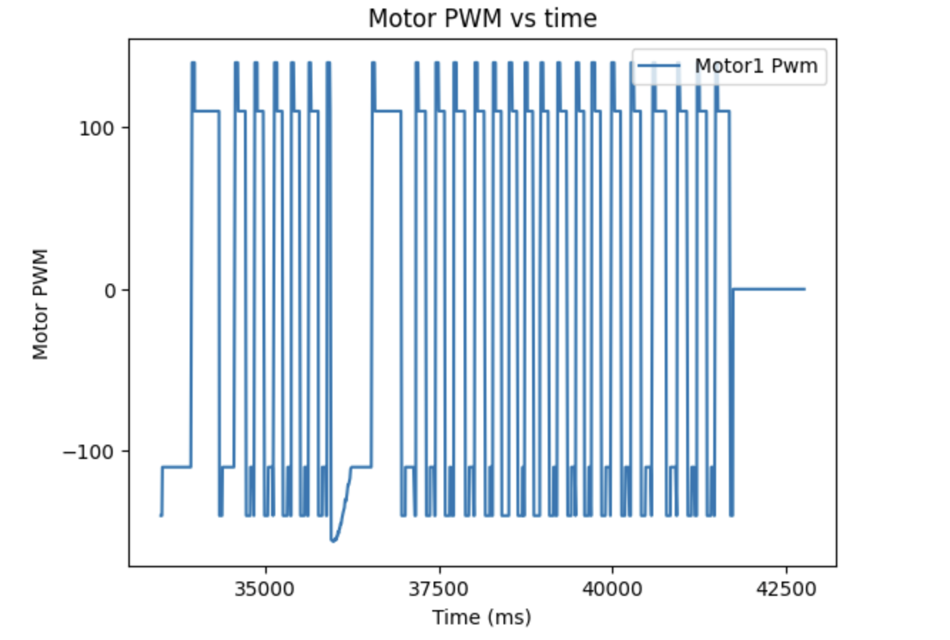
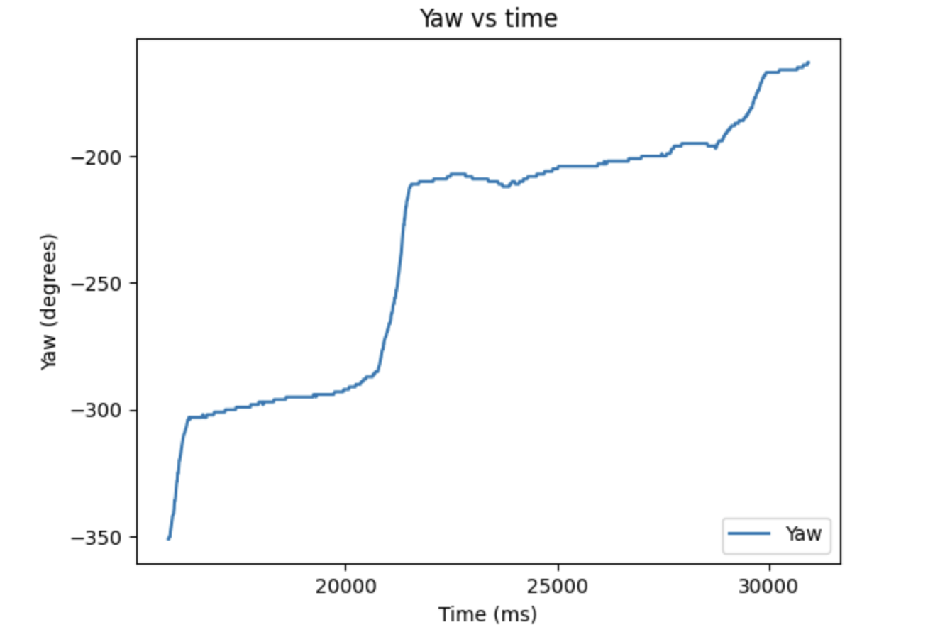
PID Control with Setpoint Change Yaw (degrees), Target Angle (degrees), and Motor Output
When the setpoint changes, the car immediately reacts and starts turning, with the yaw dropping quite quickly from 90 down to negative values, greatly overshooting the -90 target. It then corrects and oscillates around -90 degrees. This is consistent with the motor waveforms, which lowers the control to -166 when the setpoint changes, before slowing down.
5000 Level Task:
Like Lab 5, having an integrator term can lead to integrator windup, where the integral term grows too high due to the error not changing and then can not drop fast enough once it is moving. One instance this can occur is on different surfaces. The following video simulates integrator windup by having the car stuck on the backpack, and then move to a smooth floor:
The integral term wound up too high and couldn't drop quick enough, so the car kept spinning the same direction. This can be prevented by clamping the integrator term. Like lab 5, 1000 is chosen as it is high enough to allow the integral to overcome steady state error but low enough to not have windup.
                    if(mycar.I > 1000) {
                        mycar.I = 1000;
                      }
                      else if (mycar.I < -1000){
                        mycar.I = -1000;
                      }
The following video shows the same situation with the integral windup clamping.
References
I worked in the lab section on this code with Giorgi Berndt and Jorge Corpa Chunga, discussing the general approach but not specific code. I referred to both Aidan McNay and the DMP tutorial when getting the DMP to work, as well as the website of Stephen Wagner from last year.